决策树decision_tree

1 不纯度impurity

考虑特征数据集 $\mathbf{D}=(\mathbf{X},\vec{y})$ ： $$\mathbf{X}=\{\vec{x}_1, \vec{x}_2, \ldots, \vec{x}_n\} \ where \ \vec{x}_i \in \mathbb{R}^m \tag{1}$$ 每个数据点 $\vec{x}_i$ 由 $m$ 个特征组成，我们可以试着根据其中一个特征及其阈值划分数据，这样的一个划分我们称之为节点，节点是某一特征及其阈值组成的元组。

例如，假设我们有一个班的数据，这些数据中有一列是发色深色与否，我们想根据头发颜色判断男生还是女生。碰巧男生均是深色头发，女生均是浅色头发，那么我们预测深色头发为男生浅色头发为女生。那么我们只用特征深色头发与否就成功将学生性别分类了。

但是，经一个节点（也就是一个特征及其阈值）划分后每个划分的目标变量 $y$ 只含一个值的情况是理想情况。大多时候每个划分含有多个值，也就是划分后的 $y$ 的值是不纯的。比如按发色深与否划分后的两个分类，每个分类将既有男生又有女生（你见过深色头发的男生与女生，也见过浅色头发的男生与女生）。为此我们引入不纯度概念。

用于分类的不纯度impurity有：

基尼不纯度Gini impurity： $$I_{Gini}(\mathbf{D}) = \sum_k p(y=k) (1 - p(y=k)) \\ where \ k \text{ is one of all possible values of $y$} \tag{2}$$
熵不纯度Entropy impurity： $$I_{Entropy}(\mathbf{D}) = - \sum_k p(y=k) \log(p(y=k)) \\ where \ k \text{ is one of all possible values of $y$} \tag{3}$$
基尼不纯度Misclassification impurity： $$I_{Misclassification}(\mathbf{D}) = 1 - \max(p(y=k)) \\ where \ k \text{ is one of all possible values of $y$} \tag{4}$$

用于回归的不纯度impurity有：

均方差不纯度Mean Squared Error impurity： $$\begin{align}\begin{aligned}\bar{y}_m = \frac{1}{N_m} \sum_{i \in N_m} y_i\\ I_{MSE}(\mathbf{D}) = \frac{1}{N_m} \sum_{i \in N_m} (y_i - \bar{y}_m)^2\end{aligned}\end{align} \tag{5}$$
平均绝对误差不纯度Mean Absolute Error impurity： $$\begin{align}\begin{aligned}\bar{y}_m = \frac{1}{N_m} \sum_{i \in N_m} y_i\\ I_{MAE}(\mathbf{D}) = \frac{1}{N_m} \sum_{i \in N_m} |y_i - \bar{y}_m|\end{aligned}\end{align} \tag{6}$$

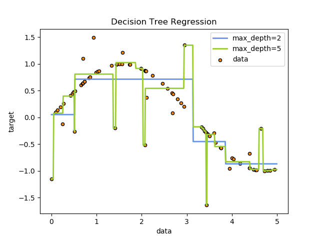
回归的不纯度impurity的应用如下图示例：回归不纯度impurity的应用

2 算法过程

数据集 $\mathbf{D}$ 经某一节点 $\sigma = \langle i, t_k \rangle$ 划分（理论是可以划分为多个区域的，但是sklearn目前仅能划分成两个区域，也就是仅能实现二分类决策Binary decisions。注意一个特征向量不一定只能有一个节点，节点由一个特征及其阈值组成，一个特征可以有多个节点。特别是回归的情况，如果只有一个特征列，经一次划分之后y的取值只有两个，回归误差定然很大，所有不可能只经一次节点划分），不纯度为： $$I(\mathbf{D},\sigma)=\frac{N_{left}}{N_\mathbf{D}}I(\mathbf{D}_{left})+\frac{N_{right}}{N_\mathbf{D}}I(\mathbf{D}_{right}) \\ where \ \mathbf{D}_{left} \cap \mathbf{D}_{right}= \varnothing \ and \ \mathbf{D}_{left} \cup \mathbf{D}_{right}= \mathbf{D}, \\ N_{left},N_{right} \text{ are the numbers of rows of $\mathbf{D}_{left}$ and $\mathbf{D}_{right}$.} \tag{7}$$ 对于数据集 $\mathbf{D}$ ，我们应该根据如下优化选择节点 $\sigma = \langle i, t_k \rangle$ ： $$\sigma^* = \operatorname{argmin}_{\sigma} I(\mathbf{D},\sigma) \tag{8}$$ 数据集 $\mathbf{D}$ 经公式(8)找到节点 $\sigma_1$ 并将数据集划分为 $\mathbf{D}_{left}$ 和 $\mathbf{D}_{right}$ ；数据集 $\mathbf{D}_{left}$ 经公式5找到节点 $\sigma_2$ 并将数据集划分为 $\mathbf{D}_{left,left}$ 和 $\mathbf{D}_{left,right}$ ；数据集 $\mathbf{D}_{right}$ 经公式(8)找到节点 $\sigma_3$ 并将数据集划分为 $\mathbf{D}_{right,left}$ 和 $\mathbf{D}_{right,right}$ ； $$\begin{align} & I(\mathbf{D},\sigma_1,\sigma_2,\sigma_3) \\ & = \frac{N_{left}}{N_\mathbf{D}}I(\mathbf{D}_{left},\sigma_2)+\frac{N_{right}}{N_\mathbf{D}}I(\mathbf{D}_{right},\sigma_3) \\ & = \frac{N_{left}}{N_\mathbf{D}}\left(\frac{N_{left,left}}{N_{left}}I(\mathbf{D}_{left,left})+\frac{N_{left,right}}{N_{left}}I(\mathbf{D}_{left,right})\right) \\ & +\frac{N_{right}}{N_\mathbf{D}}\left(\frac{N_{right,left}}{N_{right}}I(\mathbf{D}_{right,left})+\frac{N_{right,right}}{N_{right}}I(\mathbf{D}_{right,right})\right) \\ & = \frac{N_{left,left}}{N_\mathbf{D}}I(\mathbf{D}_{left,left})+\frac{N_{left,right}}{N_\mathbf{D}}I(\mathbf{D}_{left,right})+\frac{N_{right,left}}{N_\mathbf{D}}I(\mathbf{D}_{right,left}) \\ & +\frac{N_{right,right}}{N_\mathbf{D}}I(\mathbf{D}_{right,right}) \end{align} \tag{9}$$

二叉树节点数与划分后的数据集的数量之间的关系：经1次节点划分，数据集数为2；经2次节点划分，数据集数为3；……经k次节点划分，数据集数为k+1。

所以，数据集 $\mathbf{D}$ 经 $\sigma_1,\sigma_2,\ldots,\sigma_k$ 节点划分出 $\mathbf{D}_1,\mathbf{D}_2,\ldots,\mathbf{D}_{k+1}$ 等数据集，此时不纯度为： $$I(\mathbf{D},\sigma_1,\sigma_2,\ldots,\sigma_k)=\sum_{i=1}^{k+1}{\frac{N_{\mathbf{D}_{i}}}{N_\mathbf{D}}I(\mathbf{D}_{i})} \tag{10}$$ 数据集 $\mathbf{D}$ 再经 $\sigma_{k+1}$ 节点划分后数据集变为 $\mathbf{D}_1,\mathbf{D}_2,\ldots,\mathbf{D}_{k+2}$ 等数据集，此时不纯度为： $$I(\mathbf{D},\sigma_1,\sigma_2,\ldots,\sigma_k,\sigma_{k+1})=\sum_{i=1}^{k+2}{\frac{N_{\mathbf{D}_{i}}}{N_\mathbf{D}}I(\mathbf{D}_{i})} \tag{11}$$ 节点 $\sigma_{k+1}$ 的计算根据公式(8)，也就是： $$\sigma^* = \operatorname{argmin}_{\sigma_{k+1}} I(\mathbf{D},\sigma_1,\sigma_2,\ldots,\sigma_k,\sigma_{k+1}) \tag{12}$$ 到底该不该进行节点 $\sigma_{k+1}$ 划分，也就是迭代停止条件为：

1.所有节点均已纯净（即不纯度为0）
2.信息增益为0（即虽然再次节点划分仍不能保证节点纯净但节点划分前后不纯度之差为0）
3.已达最大深度（即虽然节点划分前后不纯度之差不为0但已达到参数自定义的最大深度）

3 特征重要度Feature Importance

使用多维数据集生成决策树时，评估每个特性在预测输出值方面的重要性是很有用的。在第三章，特征选择和特征工程中，我们讨论了通过只选择最重要的特征来降低数据集维数的一些方法。决策树提供了一种不同的方法，它基于每个特征所决定的不纯度下降。数据集 $\mathbf{D}$ 有 $m$ 个特征，经多个节点 $\sigma = \langle i, t_k \rangle$ 划分至满足迭代停止条件（对回归只能是达到预设深度），其中 $\sigma_1,\sigma_2,\ldots,\sigma_k$ 为根据特征列 $\vec{x}_i$ 划分，那么据特征列 $\vec{x}_i$ 的重要性可由下式计算： $${Importance}(\vec{x}_i)=\frac{\Delta{I(\vec{x}_i)}}{\sum_{i=1}^{m}{\Delta{I(\vec{x}_i)}}} \\ where \ \Delta{I(\vec{x}_i)}=\sum_{j=1}^{k}{\Delta{I(\sigma_j)}}=\sum_{j=1}^{k}{\left(\Delta{I(without \ \sigma_j)-I(with \ \sigma_j)}\right)} \tag{13}$$

特征重要度的计算涉及一个特征是不是可以由多个节点划分，迭代停止条件采用1、2还是3，因此是有点复杂的。查阅scikit-learn文档、源码，关于特征重要度的叙述是存在矛盾的，其文档中介绍无论回归和分类特征重要度的计算均基于基尼不纯度，我认为是不可能的，可能源码阅读不够深入，暂时没法确定sklearn基于什么计算特征重要度。

4 树算法：ID3、C4.5、C5.0和CART

What are all the various decision tree algorithms and how do they differ from each other? Which one is implemented in scikit-learn?的决策树算法有那些？它们之间有什么不同？scikit-learn采用哪种？

ID3 (Iterative Dichotomiser 3) was developed in 1986 by Ross Quinlan. The algorithm creates a multiway tree, finding for each node (i.e. in a greedy manner) the categorical feature that will yield the largest information gain for categorical targets. Trees are grown to their maximum size and then a pruning step is usually applied to improve the ability of the tree to generalise to unseen data. ID3(迭代二分器3)是由Ross Quinlan在1986年开发的。该算法创建了一个多路树，为每个节点(即以贪婪的方式)找到能够为分类目标带来最大信息增益的分类特征。树被长到最大的尺寸，然后修剪步骤通常被用来提高树的（泛化）能力，以推广到看不见的数据。

C4.5 is the successor to ID3 and removed the restriction that features must be categorical by dynamically defining a discrete attribute (based on numerical variables) that partitions the continuous attribute value into a discrete set of intervals. C4.5 converts the trained trees (i.e. the output of the ID3 algorithm) into sets of if-then rules. These accuracy of each rule is then evaluated to determine the order in which they should be applied. Pruning is done by removing a rule’s precondition if the accuracy of the rule improves without it. C4.5是ID3的继承者，通过动态定义一个离散属性(基于数值变量)，将连续属性值划分为一组离散的区间，消除了特征必须是分类的限制。C4.5将经过训练的树(即ID3算法的输出)转换为if-then规则集。然后，对每个规则的这些准确性进行评估，以确定应用这些规则的顺序。如果精确性在没有规则的情况下得到提高，则通过前提条件删除规则来进行修剪。

C5.0 is Quinlan’s latest version release under a proprietary license. It uses less memory and builds smaller rulesets than C4.5 while being more accurate. C5.0是Quinlan在专有许可下发布的最新版本。与C4.5相比，它使用更少的内存并构建更小的规则集，同时更准确。

CART (Classification and Regression Trees) is very similar to C4.5, but it differs in that it supports numerical target variables (regression) and does not compute rule sets. CART constructs binary trees using the feature and threshold that yield the largest information gain at each node. CART（分类和回归树）与C4.5非常相似，但它的不同之处在于它支持数值目标变量(回归)，并且不计算规则集。CART使用在每个节点上产生最大信息增益的特性和阈值构造二叉树。

scikit-learn uses an optimised version of the CART algorithm; however, scikit-learn implementation does not support categorical variables for now.scikit-learn使用了CART算法的优化版本；然而，scikit-learn实现目前不支持多分类变量（多分类特征向量）。

5 为什么决策树是弱分类器？

各个节点 $\sigma = \langle i, t_k \rangle$ 是依次依据公式(8)计算的，计算后这个节点就固定了，之后再计算节点时候前面节点无法变动。不是所有节点的联合最优。而且，每次节点划分时可以时虽然是最小化了这步的不纯度，但是最小化不存度对应的阈值和可能有多个，进而也就是对应的节点很可能有多个，特别是初始几次划分的时候。因此每个决策树的结果有很大的随机性。

6 与XGBoost，LightGBM和CatBoost之间的关系：区别和联系

参考：

sklearn文档1.10. Decision Trees；
Wiki-Decision tree learning；
[machine learning algorithms-Giuseppe Bonaccorso]()；