机器学习算法machine_learning_algorithms_1
make sure all our blog md file under post.
文前申明:机器学习算法涉及到很多公式、数学概念。为统一表述,特申明:
- 关于向量、矩阵:矩阵标记采用\mathbf{X} $\mathbf{X}$;向量标记采用 \vec{x} $\vec{x}$;行向量的元素是用逗号隔开$\vec{x} = [ x_1,x_2,\ldots,x_m ]$;列向量则用分号隔开$\vec{x} = [ x_1;x_2;\ldots;x_n ]$。
那么$n \times m$矩阵$\mathbf{X}$,可表示为由行向量作为元素组成的列向量,即:
$$\mathbf{X}=[\vec{x_1};\vec{x_2};\ldots;\vec{x_n}] \\
where \ \vec{x_i}=[x_{i1},x_{i2},\ldots,x_{im}] \\
where \ i \in \lbrace 1,2,\ldots,n \rbrace$$
那么$n \times m$矩阵$\mathbf{X}$,可表示为由列向量作为元素组成的行向量,即:
$$\mathbf{X}=[\vec{x_1},\vec{x_2},\ldots,\vec{x_m}] \\
where \ \vec{x_j}=[x_{1j};x_{2j};\ldots;x_{nj}] \\
where \ j \in \lbrace 1,2,\ldots,m \rbrace$$
区间用小括号()表示;有序的元素用中括号[],例如向量中的元素就是有顺序要求的;无序的元素用大括号{}括起来,例如集合中的元素就是不要求顺序的。
| algorithms |
|---|
监督学习、非监督学习、强化学习 分类、回归 参数学习、无参数学习
要知道这本书、这个知识的总体框架,而不一定纠结于细节。当然,若某些细节妨碍对总体框架的理解,那必须掌握他。
应该建立一个表格,把所有机器学习算法(为分清主次,先常用的)的原理、相同点、不同点、计算效率、精度、使用场合任务等等表现出来。
Machine Learning Algorithms
Giuseppe Bonaccorso
1 A Gentle Introduction to Machine Learning机器学习的简单介绍
1.1 Introduction - classic and adaptive machines介绍-经典和适应性机器
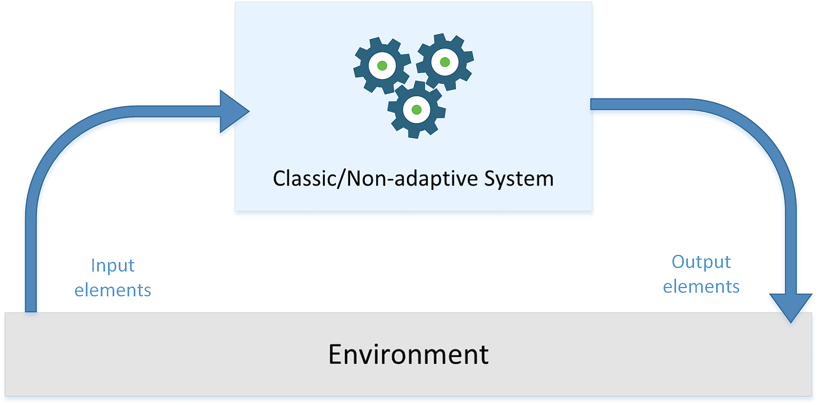
In the following figure, there's a generic representation of a classical system that receives some input values, processes them, and produces output results:在下面的图中,有一个经典系统的通用表示,它接收一些输入值,处理它们,并产生输出结果:
 Here's a schematic representation of an adaptive system:这是一个自适应系统的示意图:
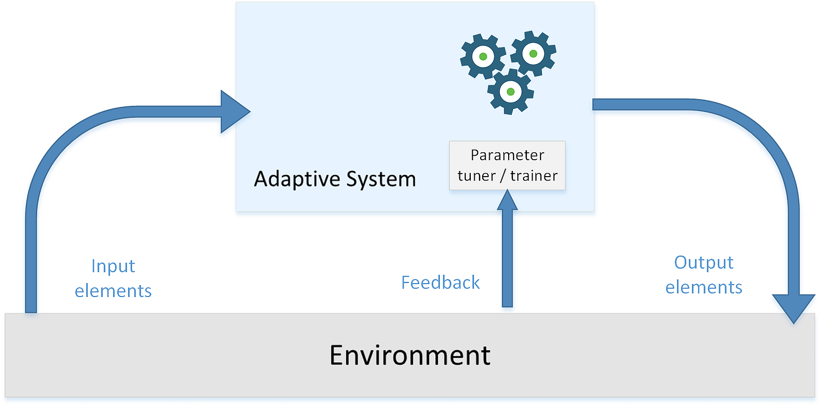 Such a system isn't based on static or permanent structures (model parameters and architectures) but rather on a continuous ability to adapt its behavior to external signals (datasets or real-time inputs) and, like a human being, to predict the future using uncertain and fragmentary pieces of information.这样的系统不是基于静态或永久性的结构(模型参数和体系结构),而是基于对外部信号(数据集或实时输入)的不断适应能力,像人类一样,利用不确定和零碎的信息预测未来。
1.2 Only learning matters只有学习才重要
What does learning exactly mean? Simply, we can say that learning is the ability to change according to external stimuli and remembering most of all previous experiences. So machine learning is an engineering approach that gives maximum importance to every technique that increases or improves the propensity for changing adaptively.学习到底意味着什么?简单地说,我们可以说学习是一种根据外界刺激而改变的能力,它能记住所有以前的经历。因此,机器学习是一种工程方法,它最大限度地重视每一项技术,以增加或改善适应变化的倾向。
1.2.1 Supervised learning监督学习
A supervised scenario is characterized by the concept of a teacher or supervisor, whose main task is to provide the agent with a precise measure of its error (directly comparable with output values).监督场景的特点基于老师或监督者,老师或监督者的主要任务是为代理提供其错误的精确度量(直接与输出值比较)。
In the following figure, a few training points are marked with circles and the thin blue line represents a perfect generalization (in this case, the connection is a simple segment):在下图中,一些训练点用圆圈标记,蓝色的细线代表完美的泛化(在本例中,连接是一个简单的分段):
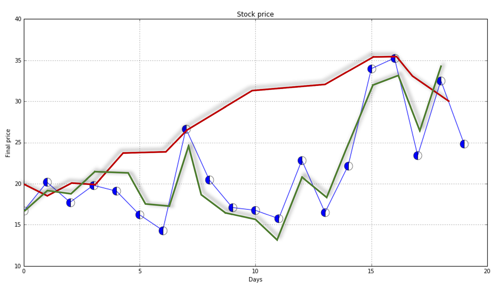 Two different models are trained with the same datasets (corresponding to the two larger lines). The former is unacceptable because it cannot generalize and capture the fastest dynamics (in terms of frequency), while the latter seems a very good compromise between the original trend and a residual ability to generalize correctly in a predictive analysis.相同数据集训练得到两个不同的模型(对应两条更粗的线条)。红线是不可接受的,因为它不能概括和捕捉最快的动态(就频率而言),而绿线似乎是原始趋势和在预测分析中正确概括的剩余能力之间的一个很好的折衷。
Formally, the previous example is called regression because it's based on continuous output values. Instead, if there is only a discrete number of possible outcomes (called categories), the process becomes a classification.前一个示例正式称为回归,因为它是基于连续输出值的。相反,如果输出值是离散数字(也叫分类),这个过程变成了一个分类。
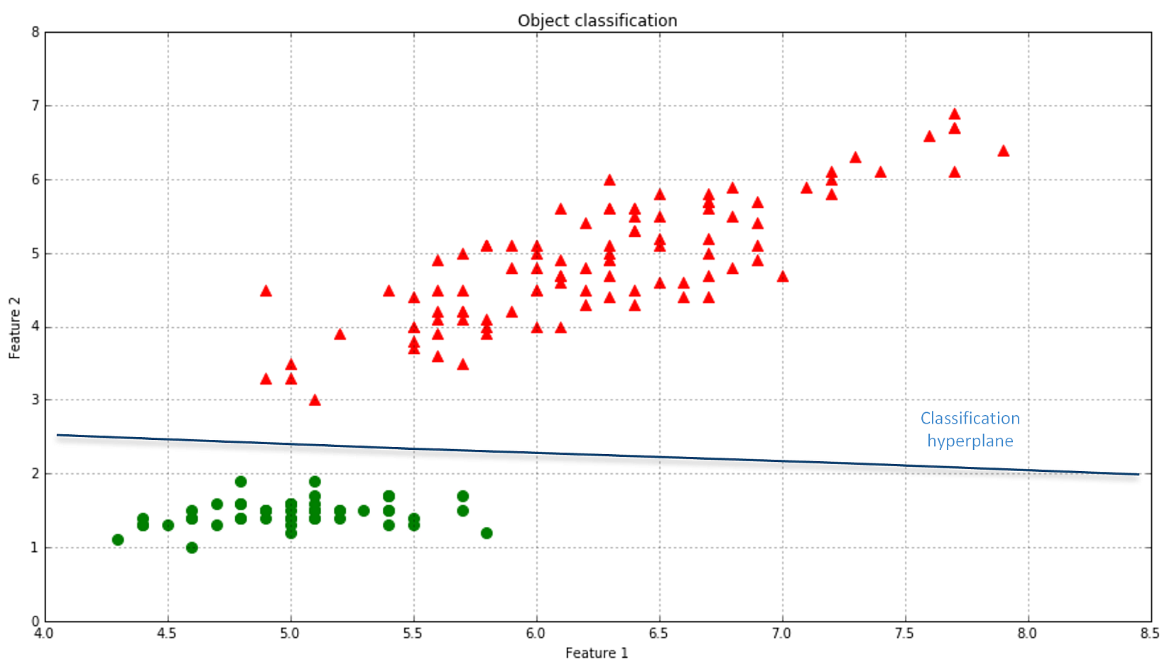
In the following figure, there's an example of classification of elements with two features. The majority of algorithms try to find the best separating hyperplane (in this case, it's a linear problem) by imposing different conditions. However, the goal is always the same: reducing the number of misclassifications and increasing the noise-robustness.在下图中,是具有两个特征的元素分类示例。大多数算法都试图通过施加不同的条件来寻找最佳的分离超平面(在这种情况下,这是一个线性问题)。但是,目标总是一样的:减少错误分类的数量,增加噪声-鲁棒性。
 Common supervised learning applications include:常见的监督学习应用包括:
1. Predictive analysis based on regression or categorical classification基于回归或分类的预测分析
2. Spam detection垃圾邮件检测
3. Pattern detection模式检测
4. Natural Language Processing自然语言处理
6. Sentiment analysis情感分析
7. Automatic image classification自动图像分类
8. Automatic sequence processing (for example, music or speech)自动序列处理(例如,音乐或语音)
1.2.2 Unsupervised learning非监督学习
This approach is based on the absence of any supervisor and therefore of absolute error measures; it's useful when it's necessary to learn how a set of elements can be grouped (clustered) according to their similarity (or distance measure).这种方法基于没有任何监督者,因此没有绝对误差测量;当需要了解如何根据一组元素的相似性(或距离度量)对它们进行分组(集群)时,这是很有用的。
In the next figure, each ellipse represents a cluster and all the points inside its area can be labeled in the same way. There are also boundary points (such as the triangles overlapping the circle area) that need a specific criterion (normally a trade-off distance measure) to determine the corresponding cluster. Just as for classification with ambiguities (P and malformed R), a good clustering approach should consider the presence of outliers and treat them so as to increase both the internal coherence (visually, this means picking a subdivision that maximizes the local density) and the separation among clusters.在下图中,每个椭圆代表一个集群,其区域内的所有点都可以以相同的方式标记。还有一些边界点(例如重叠圆形区域的三角形)需要一个特定的标准(通常是权衡距离度量)来确定相应的集群。就像模糊分类(P和畸形的R)一样,一个好的聚类方法应该考虑离群值的存在并处理它们,以增加内部一致性(视觉上,这意味着选择一个使局部密度最大化的细分)和集群间的分离度。
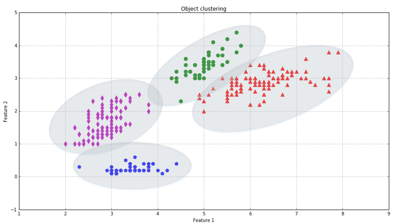
Commons unsupervised applications include:常见的非监督学习包括: 1. Object segmentation (for example, users, products, movies, songs, and so on)对象分割(例如,用户、产品、电影、歌曲等) 2. Similarity detection相似度检测 3. Automatic labeling自动标记
1.2.3 Reinforcement learning强化学习
Even if there are no actual supervisors, reinforcement learning is also based on feedback provided by the environment. However, in this case, the information is more qualitative and doesn't help the agent in determining a precise measure of its error. In reinforcement learning, this feedback is usually called reward (sometimes, a negative one is defined as a penalty) and it's useful to understand whether a certain action performed in a state is positive or not.即使没有真正的监督者,强化学习也是基于环境提供的反馈。然而,在这种情况下,信息更加定性,并不能帮助代理确定其错误的精确度量。在强化学习中,这种反馈通常被称为奖励(有时,一个消极的反馈被定义为惩罚),理解在一种状态下执行的某个行为是否为积极的是有用的。
In the following figure, there's a schematic representation of a deep neural network trained to play a famous Atari game. As input, there are one or more subsequent screenshots (this can often be enough to capture the temporal dynamics as well). They are processed using different layers (discussed briefly later) to produce an output that represents the policy for a specific state transition. After applying this policy, the game produces a feedback (as a reward-penalty), and this result is used to refine the output until it becomes stable (so the states are correctly recognized and the suggested action is always the best one) and the total reward overcomes a predefined threshold.在下面的图中,有一个训练用来玩著名的雅达利游戏的深度神经网络的示意图。作为输入,有一个或多个后续屏幕截图(这通常也足以捕获当时动态)。它们使用不同的层(稍后将简要讨论)进行处理,以生成表示特定状态转换策略的输出。在应用这个策略之后,游戏会产生一个反馈(作为奖励-惩罚),这个结果被用来完善输出,直到输出变得稳定(这样状态就被正确地识别了,并且建议的动作总是最优的),并且总回报超过了预定义的阈值。
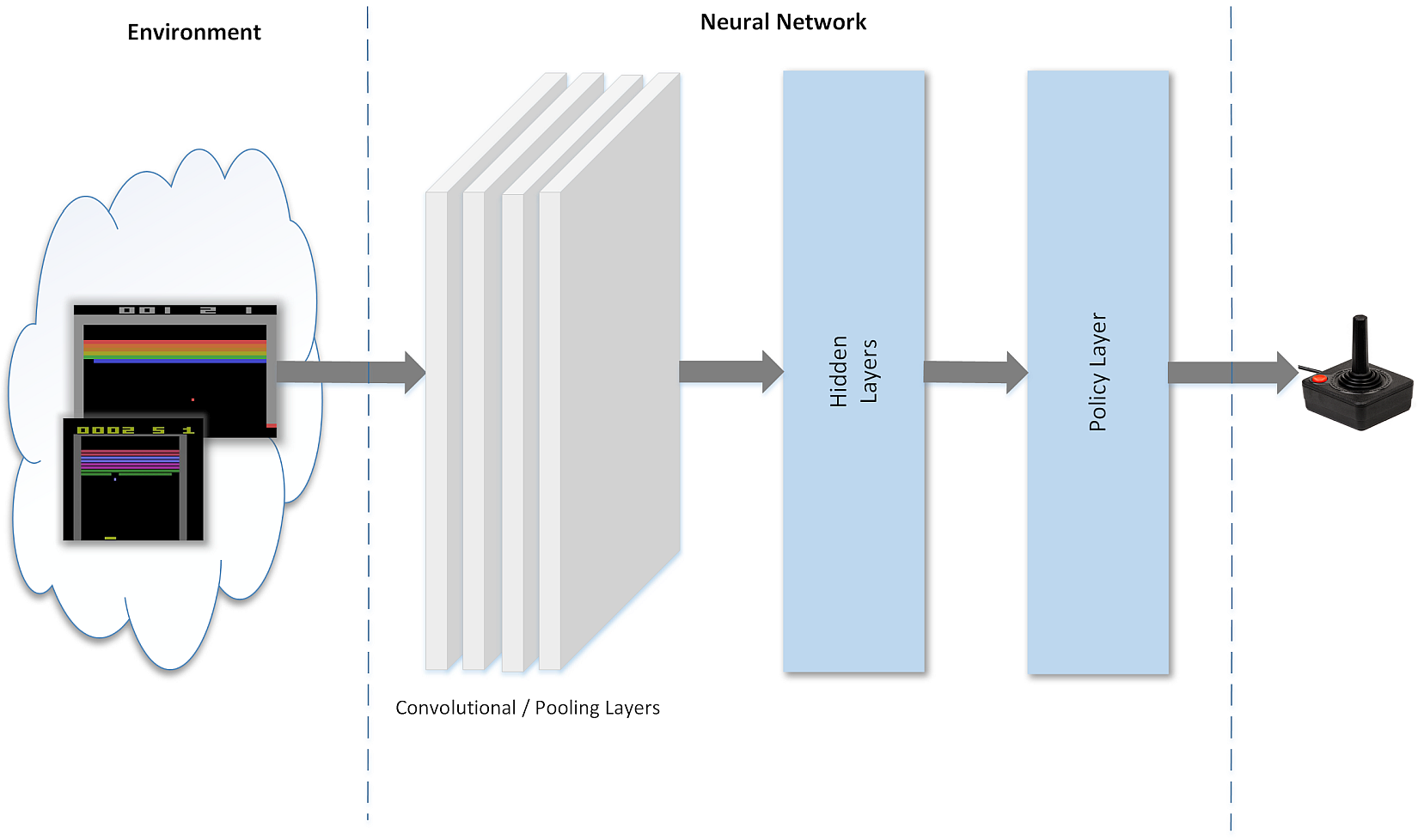
我的理解:
| 监督、非监督、强化学习 | 输入 | 原始输出 | 学习输出 | 度量标准 |
|---|---|---|---|---|
| 监督学习 | 必须有输入 | 必须有数据给出的原始输出 | 必定有预测输出 | 学习输出和原始数据输出之间的差别是客观的,但是度量标准则不是绝对的,比如线性回归可采用MSE、RMSE等各种度量。当然,应根据任务需求选择最合适的度量。 |
| 非监督学习 | 必须有输入 | 不用有数据给出的原始输出 | 必定有预测输出 | 只有学习输出而无原始数据输出,需要根据原始输入、学习输出构造度量标准;度量标准相对于监督学习更主观。 |
| 强化学习 | 必须有输入(将以图1-6代表的强化学习来举例,必须知道游戏现状。) | 不用有数据给出的原始输出(并不限定下一步动作是怎么样的) | 必定有预测输出(给出最优的建议动作) | 同样只有学习输出而无原始数据输入,同样需要根据原始输入、学习输出构造度量标准(当然,也要适应规则等),注意度量标于非监督学习仍有区别,非监督学习给出的是对总体的分值,而强化学习给出的是对总体分值的修正(奖惩)。 |
1.3 Beyond machine learning - deep learning and bio-inspired adaptive systems超越机器学习-深度学习和生物启发自适应系统
In the last decade, many researchers started training bigger and bigger models, built with several different layers (that's why this approach is called deep learning), to solve new challenging problems.在过去的十年里,许多研究者开始训练越来越大的模型,这些模型含有多个不同的层(这就是为什么这种方法被称为深度学习),以解决新的有挑战性的问题。
The idea behind these techniques is to create algorithms that work like a brain and many important advancements in this field have been achieved thanks to the contribution of neurosciences and cognitive psychology. In particular, there's a growing interest in pattern recognition and associative memories whose structure and functioning are similar to what happens in the neocortex. Such an approach also allows simpler algorithms called model-free; these aren't based on any mathematical-physical formulation of a particular problem but rather on generic learning techniques and repeating experiences.这些技术背后的理念是创造出像大脑一样工作的算法,由于神经科学和认知心理学的贡献,这一领域已经取得了许多重要的进展。特别是,人们对模式识别和联想记忆越来越感兴趣,模式识别和联想记忆的结构和功能与大脑皮层的情况类似。这种方法还允许更简单的算法,称为无模型;这些都不是基于特定问题的数学-物理公式,而是基于一般的学习技术和重复的经验。
Common deep learning applications include:常见的强化学习包括: 1. Image classification图像分类 2. Real-time visual tracking实时视觉跟踪 3. Autonomous car driving自动汽车驾驶 4. Logistic optimization物流优化 5. Bioinformatics生物信息 6. Speech recognition语音识别
1.4 Machine learning and big data机器学习与大数据
Another area that can be exploited using machine learning is big data. After the first release of Apache Hadoop, which implemented an efficient MapReduce algorithm, the amount of information managed in different business contexts grew exponentially. At the same time, the opportunity to use it for machine learning purposes arose and several applications such as mass collaborative filtering became reality.另一个可以利用机器学习的领域是大数据。在第一次发布Apache Hadoop(它实现了一种高效的MapReduce算法)之后,在不同业务上下文中管理的信息量成倍增长。与此同时,将其用于机器学习目的的机会出现了,一些应用程序如大规模协同过滤成为现实。
1.5 Further reading延伸阅读
1.6 Summary总结
2 A Important Elements in Machine Learning机器学习重要因素
a good machine learning result is normally associated with the choice of the best loss function and the usage of the right algorithm to minimize it.好的机器学习结果通常与选择最佳损失函数并采用正确的算法最小化损失函数相关联。
2.1 Data formats数据格式
In a supervised learning problem, there will always be a dataset, defined as a finite set of real vectors with m features each:监督学习问题,总会有一个数据集,定义为实数向量(行向量)组成的有限集合,每个实数向量含m个特征:

$$\mathbf{X} = \lbrace\vec{x_1};\vec{x_2};\ldots;\vec{x_n}\rbrace \ where \ \vec{x_i} \in \mathbb{R}^m$$
也就是:
$$\mathbf{X} = \lbrace\vec{x_1};\vec{x_2};\ldots;\vec{x_n}\rbrace \\
 where \ \vec{x_i} = [x_{i1},x_{i2},\ldots, x_{im}] \\
 where \ x_{ij} \in \mathbb{R}$$
为什么表示成行向量的集合用{}而不是[],因为不同的行是不同的记录,不同的列代表不同的特征,我们并不关心记录出现的先后,我们关心的是特征。
Considering that our approach is always probabilistic, we need to consider each X as drawn from a statistical multivariate distribution D. For our purposes, it's also useful to add a very important condition upon the whole dataset X: we expect all samples to be independent and identically distributed (i.i.d). This means all variables belong to the same distribution D, and considering an arbitrary subset of m values, it happens that:考虑到我们的方法总是概率,我们需要认为每个数据集X是从统计学的多变量分布D中得到的。为满足我们的目的,在整个数据集X上添加一个非常重要的条件也是很有用的;我们期待所有样本独立同分布(i.i.d)。这意味着所有变量都属于同一个分布D,考虑到m个值的任意子集,有(此时是用列向量表示):

$$P(\vec{x_1},\vec{x_2},\ldots,\vec{x_m}) = \prod_{i=1}^{m} {P(\vec{x_i})}$$
此博客环境不止怎的必须用``包裹起来方能正常显示。之后不能正确显示的话考虑加入``包裹。
The corresponding output values can be both numerical-continuous or categorical. In the first case, the process is called regression, while in the second, it is called classification. Examples of numerical outputs are:对应输出可以是连续数值或分类。如果输出是连续数值,这个过程就是回归。而如果输出是分类属性,那就叫分类。数值输出的例子如下:

$$\mathbf{y} = \lbrace y_1 ,y_2 ,\ldots, y_n \rbrace \ where \ y_i \in (0,1) \ or \ y_i \in \mathbb{R}^+$$
这里作者是说例子,并不一定要求输出为0到1之间或正实数。
Categorical examples are:分类属性输出的例子如下:

$$\mathbf{y} = \lbrace y_1 ,y_2 ,\ldots, y_n \rbrace \ where \ y_i \in \lbrace red ,black ,white, green \rbrace \ or \ y_i \in \lbrace 0, 1 \rbrace$$
We define generic regressor, a vector-valued function which associates an input value to a continuous output and generic classifier, a vector-values function whose predicted output is categorical (discrete). If they also depend on an internal parameter vector which determines the actual instance of a generic predictor, the approach is called parametric learning:我们定义通用回归器,一个将输入值与连续输出关联的向量值函数;和一个通用分类器,一个预测输出为分类(离散的)的向量值函数。如果它们也靠内部参数向量来决定通用预测器的实际实例,这个方法称为参数学习:

$$\tilde{y} = r(\vec{x}, \vec{\theta}) \\
\tilde{y} = c(\vec{x}, \vec{\theta}) \\
where \ \vec{\theta} \ is \ the \ generic \ internel \ parameter \ vector$$
On the other hand, non-parametric learning doesn't make initial assumptions about the family of predictors (for example, defining a generic parameterized version of r(...) and c(...)). A very common non-parametric family is called instance-based learning and makes real-time predictions (without pre-computing parameter values) based on hypothesis determined only by the training samples (instance set). A simple and widespread approach adopts the concept of neighborhoods (with a fixed radius). In a classification problem, a new sample is automatically surrounded by classified training elements and the output class is determined considering the preponderant one in the neighborhood. kernel-based support vector machines are another very important algorithm family belonging to this class.相反,无参数学习并没有对预测器做初始假设(例如,例如,定义r(...)和c(...)的通用参数化版本)。一个非常常见的非参数族称为基于实例的学习,它基于仅由训练样本(实例集)确定的假设进行实时预测(不需要预计算参数值)。一种简单而广泛的方法采用了临近关系的概念(具有固定的半径)。在分类问题中,一个新的样本被已归类的训练元素自动包围,且输出分类参考占优势的临近关系来确定。基于核的支持向量机(kernel-based support vector machines)是另一种无参数学习的算法。
A generic parametric training process must find the best parameter vector which minimizes the regression error given a specific training dataset and it should also generate a predictor that can correctly generalize when unknown samples are provided.一般的参数训练过程必须找到在给定特定训练数据集的情况下使回/分类归误差最小化的最佳参数向量,并生成一个预测器,在提供未知样本时能够正确推广。显然,无参数的学习也是要优化什么?????以使误差最小化并可推广。抱歉,暂时不知道无参数的学习中对应参数学习中的参数的是什么。
Another interpretation can be expressed in terms of additive noise:另一个解释可表达为附加的噪声:
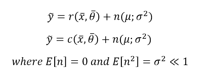
$$\tilde{y} = r(\vec{x}, \vec{\theta}) + n(\mu;{\sigma}^2) \\
\tilde{y} = c(\vec{x}, \vec{\theta}) + n(\mu;{\sigma}^2) \\
where \ E(n)=\mu=0 \ and \ E(n^{2})={\sigma}^2 \ll 1$$
For our purposes, we can expect zero-mean and low-variance Gaussian noise added to a perfect prediction. A training task must increase the signal-noise ratio by optimizing the parameters. Of course, whenever such a term doesn't have zero mean (independently from the other X values), probably it means that there's a hidden trend that must be taken into account (maybe a feature that has been prematurely discarded). On the other hand, high noise variance means that X is dirty and its measures are not reliable.为满足我们的目的,我们期望零均值和低方差的高斯噪声来完美预测。训练任务必须通过优化参数来提高信噪比。当然,当这样一个项没有零平均值(独立于其他X值)时,可能意味着还有一个隐藏的趋势(可能是一个被过早丢弃的特性)必须考虑到。另一方面,高噪声方差意味着X是脏的,其测量不可靠。显然,无参数的学习也是要优化什么?????以使信噪比最大
In unsupervised learning, we normally only have an input set X with m-length vectors, and we define clustering function (with n target clusters) with the following expression:在无监督学习中,我们通常只有一个长度为m的向量的输入集X,我们用下面的表达式定义聚类函数(有n个目标簇):

$$k_t = c(\vec{x}, \vec{\theta}) \ where \ k_t \in \lbrace 1,2,\ldots,n \rbrace$$
2.1.1 Multiclass strategies分类策略
When the number of output classes is greater than one, there are two main possibilities to manage a classification problem:当输出分类的数量大于1时,管理分类问题有两种主要的可能性 * One-vs-all一对多 * One-vs-one一对一
2.1.1.1 One-vs-all一对多
This is probably the most common strategy and is widely adopted by scikit-learn for most of its algorithms. If there are n output classes, n classifiers will be trained in parallel considering there is always a separation between an actual class and the remaining ones. This approach is relatively lightweight (at most, n-1 checks are needed to find the right class, so it has an O(n) complexity) and, for this reason, it's normally the default choice and there's no need for further actions.这可能是最常见的策略,并被scikit-learn的大多数算法广泛采用。如果有n个输出分类,考虑到实际分类和剩余分类之间总是存在间隔,将会并行训练n个分类器。这种方法是相对轻量级的(找到正确的分类最多需要n-1次检查,因此它具有O(n)复杂性),因此,它通常是默认选择,不需要进一步的操作。
Multiclass as One-Vs-All:
- sklearn.ensemble.GradientBoostingClassifier
- sklearn.gaussian_process.GaussianProcessClassifier (setting multi_class = “one_vs_rest”)
- sklearn.svm.LinearSVC (setting multi_class=”ovr”)
- sklearn.linear_model.LogisticRegression (setting multi_class=”ovr”)
- sklearn.linear_model.LogisticRegressionCV (setting multi_class=”ovr”)
- sklearn.linear_model.SGDClassifier
- sklearn.linear_model.Perceptron
- sklearn.linear_model.PassiveAggressiveClassifier
2.1.1.1 One-vs-one一对一
The alternative to one-vs-all is training a model for each pair of classes. The complexity is no longer linear (it's $O(n^2)$ indeed) and the right class is determined by a majority vote. In general, this choice is more expensive and should be adopted only when a full dataset comparison is not preferable.另一种方法是一对一,即每队分类训练一个模型。复杂度不再是线性的(而是$O(n^2)$),并且正确的分类取决于大多数投票结果。一般来说,这种选择比较昂贵,只有当完整的数据集比较不可取时才应该采用。
Multiclass as One-Vs-One:
- sklearn.svm.NuSVC
- sklearn.svm.SVC.
- sklearn.gaussian_process.GaussianProcessClassifier (setting multi_class = “one_vs_one”)
2.2 Learnability可学习性
A parametric model can be split into two parts: a static structure and a dynamic set of parameters. The former is determined by choice of a specific algorithm and is normally immutable (except in the cases when the model provides some re-modeling functionalities), while the latter is the objective of our optimization. Considering n unbounded parameters, they generate an n-dimensional space (imposing bounds results in a sub-space without relevant changes in our discussion) where each point, together with the immutable part of the estimator function, represents a learning hypothesis H (associated with a specific set of parameters):参数模型可分为两部分:一种静态结构和一组动态参数。前者由特定算法的选择决定,通常是不可变的(除非模型提供一些重新建模功能),而后者是我们优化的目标。考虑到n个无界参数,它们会生成一个n维空间(在我们的讨论中,在没有相关更改的情况下,将边界设置在子空间中),空间中每个点与估计函数的不可变部分一起表示一个学习假设H(与一组特定参数相关联):

$$\mathbf{H} = [{\theta}_{1},{\theta}_{2},\ldots,{\theta}_{n}]$$
各参数之间肯定是有顺序的,所以我改用[]表示。不要因此认为参数个数与数据点个数相等!
In the following figure, there's an example of a dataset whose points must be classified as red (Class A) or blue (Class B). Three hypotheses are shown: the first one (the middle line starting from left) misclassifies one sample, while the lower and upper ones misclassify 13 and 23 samples respectively:在下面的图中,有一个数据集的示例,其点必须分类为红色(类a)或蓝色(类B)。有三个假设:第一个假设(左起中间的线条)对1个样本进行了错误分类,而下面的假设和上面的假设分别对13个样本和23个样本进行了错误分类:
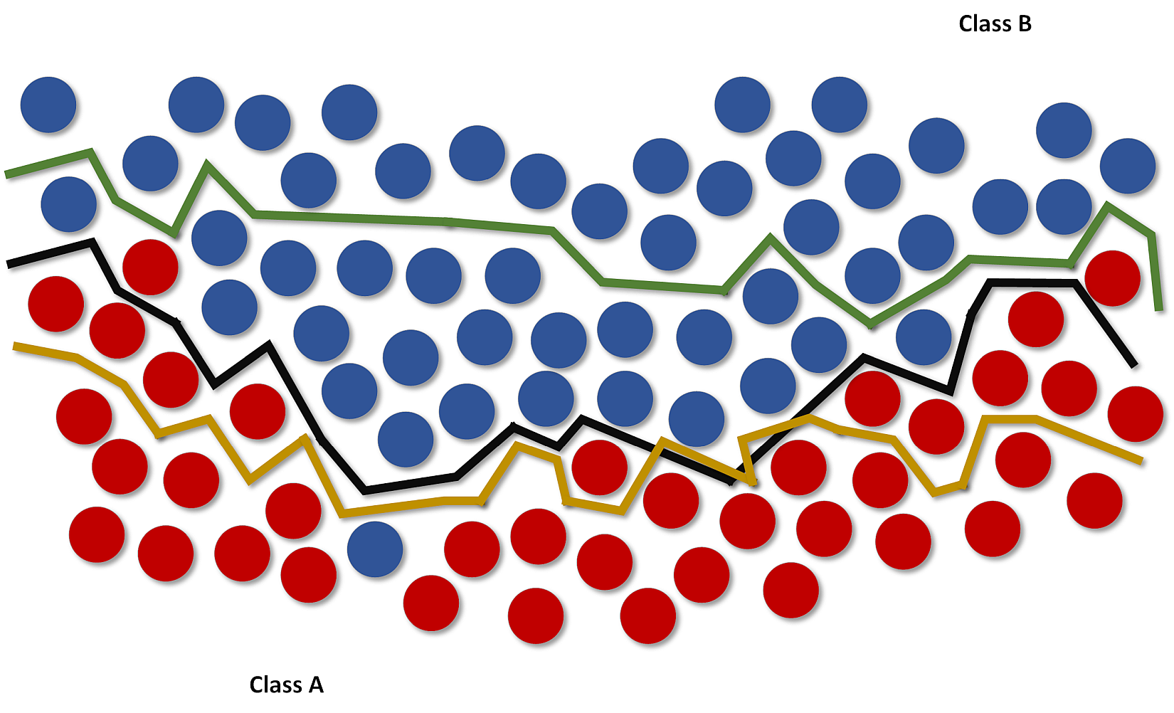 We say that the dataset X is linearly separable (without transformations) if there exists a hyperplane which divides the space into two subspaces containing only elements belonging to the same class.如果存在超平面,它将空间分成两个子空间,子空间只包含属于同一个类的元素,我们就说数据集X是线性可分的(没有变换)。
Consider the example shown in the following figure:考虑下图的例子:
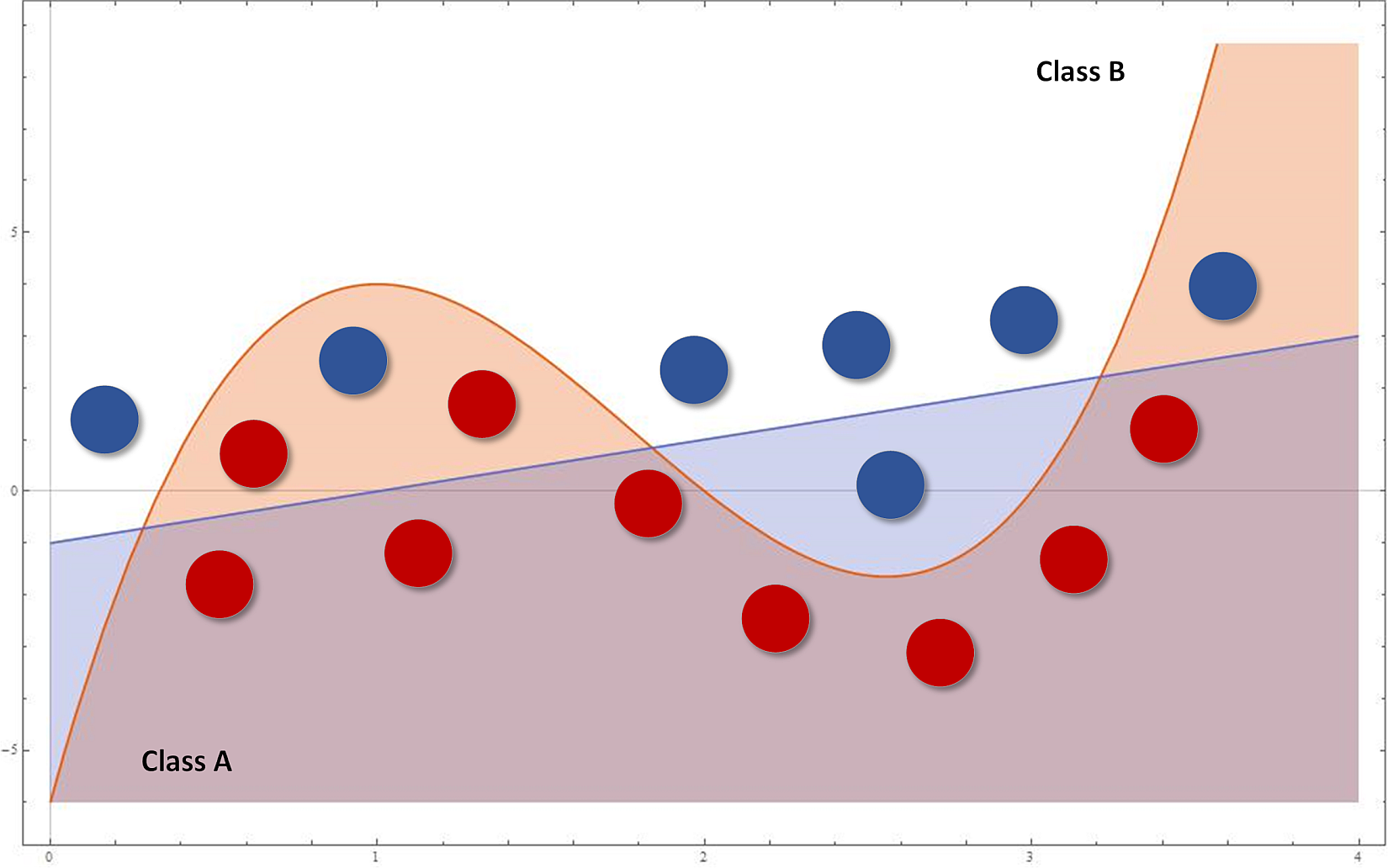 The blue classifier is linear while the red one is cubic. At a glance, non-linear strategy seems to perform better, because it can capture more expressivity, thanks to its concavities. However, if new samples are added following the trend defined by the last four ones (from the right), they'll be completely misclassified. In fact, while a linear function is globally better but cannot capture the initial oscillation between 0 and 4, a cubic approach can fit this data almost perfectly but, at the same time, loses its ability to keep a global linear trend. Therefore, there are two possibilities:蓝色分类器是线性的而红色的是三次方的。乍一看,非线性策略似乎表现得更好,因为它可以捕捉到更多的表现力,这要归功于它的复杂性。但是,如果按照最后四个(从右边)定义的趋势添加新样本,它们将完全被错误分类。实际上,虽然线性函数在全局上更好,但不能捕捉到0和4之间的初始振荡,但三次方的方法可以几乎完美地拟合这些数据,但同时,失去了保持全局线性趋势的能力。有两种可能性:
- If we expect future data to be exactly distributed as training samples, a more complex model can be a good choice, to capture small variations that a lower-level one will discard. In this case, a linear (or lower-level) model will drive to underfitting, because it won't be able to capture an appropriate level of expressivity.如果我们期望未来的数据与训练数据完全一样分布,那么一个更复杂的模型可能是一个不错的选择,它可以捕获指数较低的模型将丢弃的小变动。在这种情况下,线性(或指数较低)模型会导致欠拟合,因为它无法捕捉到合适的表达水平。
- If we think that future data can be locally distributed differently but keeps a global trend, it's preferable to have a higher residual misclassification error as well as a more precise generalization ability. Using a bigger model focusing only on training data can drive to overfitting.如果我们认为未来的数据可能会局趋势相同但局部分布不同,那么最好是有更高的残差分类误差和更精确的泛化能力。使用一个只关注训练数据的更大的模型会导致过拟合。
2.2.1 Underfitting and overfitting欠拟合和过拟合
The purpose of a machine learning model is to approximate an unknown function that associates input elements to output ones (for a classifier, we call them classes). Unfortunately, this ideal condition is not always easy to find and it's important to consider two different dangers:机器学习模型的目的是近似一个未知函数,该函数将输入元素与输出元素关联起来(对于分类器,我们将其称为类)。不幸的是,这种理想状态并不总是容易找到的,考虑两种不同的危险是很重要的:
- Underfitting: It means that the model isn't able to capture the dynamics shown by the same training set (probably because its capacity is too limited).欠拟合:即模型不能捕捉训练集表现出的动态(很可能因为模型能力有限)。
- Overfitting: the model has an excessive capacity and it's not more able to generalize considering the original dynamics provided by the training set. It can associate almost perfectly all the known samples to the corresponding output values, but when an unknown input is presented, the corresponding prediction error can be very high.过拟合:即模型能力过大,因为(过多)考虑到训练集提供的原始动态,它并不能更泛化。它几乎可以将所有已知的样本与相应的输出值完美地关联起来,但当出现未知输入时,相应的预测误差可能非常高。
In the following picture, there are examples of interpolation with low-capacity (underfitting), normal-capacity (normal fitting), and excessive capacity (overfitting):下图中,是低能力(欠拟合)、正常能力(正常拟合)和过高能力(过拟合)插值的例子:
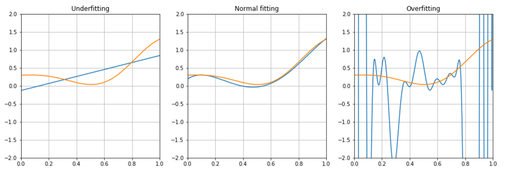 Underfitting is easier to detect considering the prediction error, while overfitting may prove to be more difficult to discover as it could be initially considered the result of a perfect fitting.考虑到预测误差,欠拟合更容易检测,而过度拟合可能被证明更难发现,因为它本来最初被认为是一个完美拟合的结果。
Cross-validation and other techniques that we're going to discuss in the next chapters can easily show how our model works with test samples never seen during the training phase. That way, it would be possible to assess the generalization ability in a broader context (remember that we're not working with all possible values, but always with a subset that should reflect the original distribution).交叉验证和我们将在下一章中讨论的其他技术可以很容易地展示我们的模型在训练阶段未见过的测试样本情况下表现如何。这样,就有可能在更广泛的背景下评估泛化能力(请记住,我们并不是使用所有可能的值,而是始终使用一个反映原始分布的子集)。
However, a generic rule of thumb says that a residual error is always necessary to guarantee a good generalization ability, while a model that shows a validation accuracy of 99.999... percent on training samples is almost surely overfitted and will likely be unable to predict correctly when never-seen input samples are provided.然而,一个通用的经验法则说,为了保证良好的泛化能力,残差总是必要的,而一个在训练样本上验证精度为99.999……百分比的模型几乎肯定是过拟合的,并且可能无法对提供的未见输入样本进行正确预测。
2.2.2 Error measures误差度量
In general, when working with a supervised scenario, we define a non-negative error measure $e_m$ which takes two arguments (expected and predicted output) and allows us to compute a total error value over the whole dataset (made up of n samples):通常,在使用有监督场景时,我们定义一个非负误差度量$e_m$,它接受两个参数(预期输出和预期输出),并允许我们计算整个数据集(由n个样本组成)的总误差值:

$${Error}_{H}=\sum_{i=1}^{n} {e_{m}(\tilde{y_{i}},y_{i})} \ where \ e_{m} \ge 0 \ \forall \ \tilde{y_{i}},y_{i}$$
This value is also implicitly dependent on the specific hypothesis H through the parameter set, therefore optimizing the error implies finding an optimal hypothesis (considering the hardness of many optimization problems, this is not the absolute best one, but an acceptable approximation). In many cases, it's useful to consider the mean square error (MSE):这个值也通过参数集隐含地依赖于特定的假设H,因此优化误差意味着找到一个最优假设(考虑到许多优化问题的难度,这不是绝对最好的,而是一个可接受的近似)。在许多情况下,考虑均方误差(MSE)是很有用的:
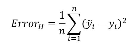
$${Error}_{H}=\frac{1} {n} \sum_{i=1}^{n} {(\tilde{y_{i}} - y_{i})^2}$$
Its initial value represents a starting point over the surface of a n-variables function. A generic training algorithm has to find the global minimum or a point quite close to it (there's always a tolerance to avoid an excessive number of iterations and a consequent risk of overfitting). This measure is also called loss function because its value must be minimized through an optimization problem. When it's easy to determine an element which must be maximized, the corresponding loss function will be its reciprocal.它的初始值表示一个n变量函数表面的起点。一个通用的训练算法必须找到全局最小值或非常接近它的点(总是要有一个容忍度来避免过多的迭代和随之而来的过度拟合风险)。这种度量也称为损失函数,因为它的值必须通过优化问题最小化。当很容易确定一个必须最大化的元素时,相应的损失函数将是它的倒数(或负值,这样损失函数仍可通过最小化来优化)。
Another useful loss function is called zero-one-loss and it's particularly efficient for binary classifications (also for one-vs-rest multiclass strategy):另一有用损失函数叫零一损失,特别对二分类问题(也对一对多多分类策略)特别有效:

$${L}_{0/1H}(\tilde{y_{i}},y_{i})=\begin{cases} 0, & \text{if $\tilde{y_{i}} = y_{i}$} \\ 1, & \text{if $\tilde{y_{i}} \ne y_{i}$} \end{cases}$$
This function is implicitly an indicator and can be easily adopted in loss functions based on the probability of misclassification.该函数是一个隐式的指示器,在基于误分类概率的损失函数中很容易使用。
A helpful interpretation of a generic (and continuous) loss function can be expressed in terms of potential energy:一个通用的(连续的)损失函数的有用解释可以用势能项来表示:

$${Energy}_{H}=\frac{1} {2} \sum_{i=1}^{n} {{e_{m}}^2(\tilde{y_{i}} , y_{i})}$$
The predictor is like a ball upon a rough surface: starting from a random point where energy (=error) is usually rather high, it must move until it reaches a stable equilibrium point where its energy (relative to the global minimum) is null. In the following figure, there's a schematic representation of some different situations:预测器犹如粗糙表面上的球:从能量(也就是误差)通常相当高的随机点开始,移动到能量为零(相对全局最小)的稳定的平衡点方止。下图中,有一些不同情况的示意图:
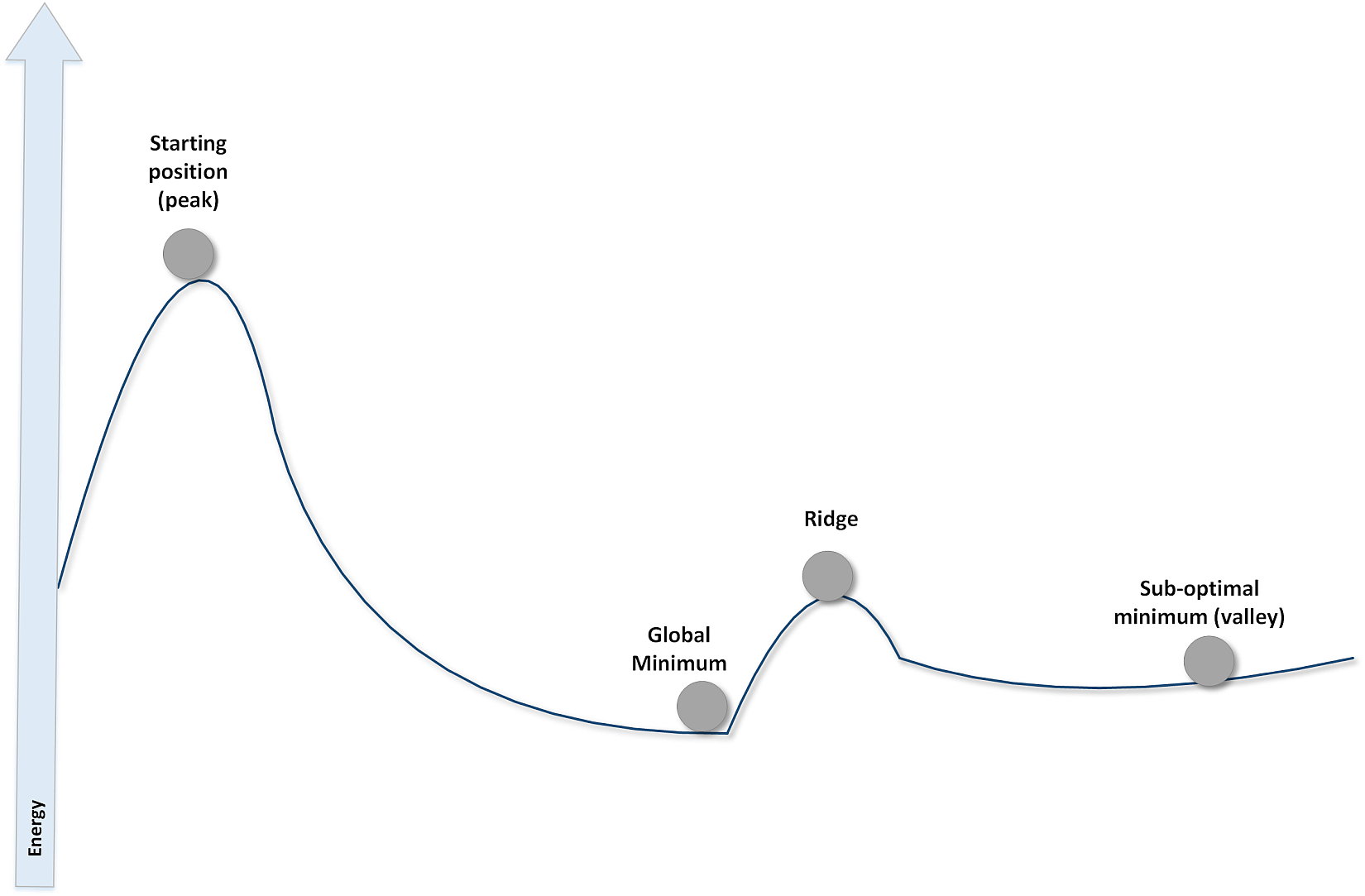 Just like in the physical situation, the starting point is stable without any external perturbation, so to start the process, it's needed to provide initial kinetic energy. However, if such an energy is strong enough, then after descending over the slope the ball cannot stop in the global minimum. The residual kinetic energy can be enough to overcome the ridge and reach the right valley. If there are not other energy sources, the ball gets trapped in the plain valley and cannot move anymore. There are many techniques that have been engineered to solve this problem and avoid local minima. However, every situation must always be carefully analyzed to understand what level of residual energy (or error) is acceptable, or whether it's better to adopt a different strategy.就像在物理情况下,起始点是稳定的,没有任何外部扰动,所以要开始这个过程,需要提供初始动能。然而,如果这样的能量足够强大,那么在下降到斜坡之后,球就不能在全球最小值停止。剩余动能足以克服山脊,到达右边的山谷。如果没有其他能源,球就会被困在平缓的山谷,无法移动。有许多技术已经被设计来解决这个问题并避免局部极小值。然而,每一种情况都必须仔细分析,以了解什么程度的剩余能量(或误差)是可以接受的,或者采用不同的策略是否更好。
注意到误差公式和能量公式之间的关系了吗?不考虑求和记号,其实后者求导即得前者。
2.2.3 PAC learning PAC学习理论
In many cases machine learning seems to work seamlessly, but is there any way to determine formally the learnability of a concept? In 1984, the computer scientist L. Valiant proposed a mathematical approach to determine whether a problem is learnable by a computer. The name of this technique is PAC, or probably approximately correct.在许多情况下,机器学习似乎可以无缝地工作,但有什么方法可以正式确定一个概念的可学性?1984年,计算机科学家L. Valiant提出了一种数学方法来确定问题是否可以通过计算机学习。这种技术叫可能近似正确(PAC)。
The original formulation (you can read it in Valiant L., A Theory of the Learnable, Communications of the ACM, Vol. 27, No. 11 , Nov. 1984) is based on a particular hypothesis, however, without a considerable loss of precision, we can think about a classification problem where an algorithm A has to learn a set of concepts. In particular, a concept is a subset of input patterns X which determine the same output element. Therefore, learning a concept (parametrically) means minimizing the corresponding loss function restricted to a specific class, while learning all possible concepts (belonging to the same universe), means finding the minimum of a global loss function.最初的公式(你可从Valiant L., A Theory of the Learnable, Communications of the ACM, Vol. 27, No. 11 , Nov. 1984阅读)是基于一个特定的假设,然而,在没有很大的精度损失的情况下,我们可以考虑一个分类问题,其中算法A必须学习一组概念。特别是,概念是输入模式X的子集,X决定相同输出元素。因此,学习一个概念(参数化)意味着将相应的损失函数限制在一个特定的分类中,而学习所有可能的概念(属于同一个全局)意味着找到全局损失函数的最小值。
However, given a problem, we have many possible (sometimes, theoretically infinite) hypotheses and a probabilistic trade-off is often necessary. For this reason, we accept good approximations with high probability based on a limited number of input elements and produced in polynomial time.然而,给定一个问题,我们有许多可能的(有时,理论上是无限的)假设,一个概率权衡通常是必要的。因此,我们接受基于有限数量输入元素并在多项式时间内产生的高概率近似。
Therefore, an algorithm A can learn the class C of all concepts (making them PAC learnable) if it's able to find a hypothesis H with a procedure $O(n^k)$ so that A, with a probability p, can classify all patterns correctly with a maximum allowed error $m_e$. This must be valid for all statistical distributions on X and for a number of training samples which must be greater than or equal to a minimum value depending only on p and me.因此,如果算法能够通过过程$O(n^k)$找到假设H,那么A,在概率p的情况下,可以用最大允许误差$m_e$正确地分类所有模式,那么一个算法A可以学习所有概念构成的分类C(使它们成为PAC可学习的)。
The constraint to computation complexity is not a secondary matter, in fact, we expect our algorithms to learn efficiently in a reasonable time also when the problem is quite complex. An exponential time could lead to computational explosions when the datasets are too large or the optimization starting point is very far from an acceptable minimum. Moreover, it's important to remember the so-called curse of dimensionality, which is an effect that often happens in some models where training or prediction time is proportional (not always linearly) to the dimensions, so when the number of features increases, the performance of the models (that can be reasonable when the input dimensionality is small) gets dramatically reduced. Moreover, in many cases, in order to capture the full expressivity, it's necessary to have a very large dataset and without enough training data, the approximation can become problematic (this is called Hughes phenomenon). For these reasons, looking for polynomial-time algorithms is more than a simple effort, because it can determine the success or the failure of a machine learning problem. For these reasons, in the next chapters, we're going to introduce some techniques that can be used to efficiently reduce the dimensionality of a dataset without a problematic loss of information.计算复杂度的限制并不是次要问题,事实上,当问题相当复杂的时候,我们希望我们的算法在合理的时间内高效地学习。当数据集太大或者优化起点离可接受的最小值太远时,指数级时间可能导致计算爆炸。此外,重要的是要记住所谓的维度诅咒,训练和预测时间与维度成正比(不总是线性)的模型经常有这类问题,所以当特征数量的增加,模型的性能(输入维度小时模型的性能才合理)被大大降低了。此外,在许多情况下,为了获得完整的表达能力,需要有一个非常大的数据集,而没有足够的训练数据,近似就会成为问题(这被称为休斯现象)。由于这些原因,寻找多项式时间算法不仅仅是一项简单的工作,因为它可以决定机器学习问题的成败。为防止维度诅咒和休斯现象,需要在不损失信息的前提下有效降低维度。
我的总结:进行T次运算,以p的概率实现$m_e$的误差实现算法A,如果T不大于$O(n^k)$且p和$m_e$可框定范围,那么算法A就是分类C(分类C包含算法A的全部可能的概念或者说可能的参数)的PAC可学算法。
2.3 Statistical learning approaches统计学习法
Imagine that you need to design a spam-filtering algorithm starting from this initial (over-simplistic) classification based on two parameters:假设您需要设计一个基于两个参数的初始(过于简单)分类的垃圾邮件过滤算法:
| Parameter | Spam emails (X1) | Regular emails (X2) |
|---|---|---|
| p1 - Contains > 5 blacklisted words | 80 | 20 |
| p2 - Message length < 20 characters | 75 | 25 |
We have collected 200 email messages (X) (for simplicity, we consider p1 and p2 mutually exclusive) and we need to find a couple of probabilistic hypotheses (expressed in terms of p1 and p2), to determine:我们收集了200封电子邮件(X)(为了简单起见,我们认为p1和p2互斥,只为了保证上表和刚好为200,无其他意义。),我们需要找到一对概率假设(用p1和p2表示)来确定:

$$P(spam \mid h_{p1}, h_{p2})$$
We also assume the conditional independence of both terms (it means that $h_{p1}$ and $h_{p2}$ contribute conjunctly to spam in the same way as they were alone).我们还假设这两项都是条件独立的(这意味着$h_{p1}$和$h_{p2}$以单独的方式共同导致垃圾邮件)。
For example, we could think about rules (hypotheses) like: "If there are more than five blacklisted words" or "If the message is less than 20 characters in length" then "the probability of spam is high" (for example, greater than 50 percent). However, without assigning probabilities, it's difficult to generalize when the dataset changes (like in a real world antispam filter). We also want to determine a partitioning threshold (such as green, yellow, and red signals) to help the user in deciding what to keep and what to trash.例如,我们可想象规则(假设)如:“若有超过超过5个黑名单单词”或“若信息长度少于20字符”那么“是垃圾邮件的可能性高”(例如,超过50%)。但是,如果不分配概率,就很难在数据集发生变化时进行概括(就像在实际的反垃圾邮件过滤器中那样)。我们还希望确定分区阈值(例如绿色、黄色和红色信号),以帮助用户决定保留哪些内容和销毁哪些内容。
As the hypotheses are determined through the dataset $\mathbf{X}$, we can also write (in a discrete form):由于假设是通过数据集$\mathbf{X}$确定的,我们还可以(以离散形式)写成:

$$P(spam \mid \mathbf{X})=\sum_{i} {P(spam \mid h_{pi})P(h_{pi} \mid \mathbf{X})}$$
【
记$A=spam \mid \mathbf{X}$并$B_{i}=h_{pi} \mid \mathbf{X}$,若$B_{i}$的全体组成完备事件组,即它们两两互不相容,其和为全集,那么由全概率公式:
$$P(A)=\sum_{i} {P(A \mid B_{i})P(B_{i})}$$
即:
$$P(spam \mid \mathbf{X})=\sum_{i} {P(spam \mid h_{pi})P(h_{pi} \mid \mathbf{X})}$$
注意:条件p1与p2互斥则其两者不可能独立,作者原文是p1的条件概率与p2的条件概率互斥。 】
【 公式右边,第一项很好求,就如上表。公式第二项可以采用以下3种方法:
贝叶斯方法。假设多时很耗时,因为要穷尽计算每一项然后求和。
MAP learning。根据后验概率选择最可能的假设,其他假设忽略。缺点是依赖于先验概率。
Maximum-likelihood learning。即用极大似然代替。
此备注暂留,但由于摘抄时未详细信息,已不知道所指是何公式了。 】
In this example, it's quite easy to determine the value of each term. However, in general, it's necessary to introduce the Bayes formula (which will be discussed in Chapter 6, Naive Bayes):这个例子中,决定每项的值很容易。然而,引入贝叶斯公式是必要的(将在第六章讨论)。

$$P(h_{pi} \mid \mathbf{X}) \propto P(\mathbf{X} \mid h_{pi})P(h_{pi})$$
The proportionality is necessary to avoid the introduction of the marginal probability P(X), which acts only as a normalization factor (remember that in a discrete random variable, the sum of all possible probability outcomes must be equal to 1).为了避免引入边际概率P(X),比例是必要的。边际概率P(X)仅作为一个标准化因子(记住,在离散随机变量中,所有可能的概率结果之和必须等于1)。
In the previous equation, the first term is called a posteriori (which comes after) probability, because it's determined by a marginal Apriori (which comes first) probability multiplied by a factor which is called likelihood. To understand the philosophy of such an approach, it's useful to take a simple example: tossing a fair coin. Everybody knows that the marginal probability of each face is equal to 0.5, but who decided that? It's a theoretical consequence of logic and probability axioms (a good physicist would say that it's never 0.5 because of several factors that we simply discard). After tossing the coin 100 times, we observe the outcomes and, surprisingly, we discover that the ratio between heads and tails is slightly different (for example, 0.46). How can we correct our estimation? The term called likelihood measures how much our actual experiments confirm the Apriori hypothesis and determines another probability (a posteriori) which reflects the actual situation. The likelihood, therefore, helps us in correcting our estimation dynamically, overcoming the problem of a fixed probability.在前面的方程中,第一项被称为后验概率(因为已见数据),因为它是由边际先验概率(因为没见数据)乘以一个被称为似然的因子决定的。要理解这种方法的哲学,我们可以举一个简单的例子:抛一枚均匀的硬币。大家都知道每个面的边际概率是0.5,但谁决定的?这是逻辑和概率公理的一个理论推论(一个好的物理学家会说,它永远不会是0.5,因为有几个因素我们只是简单地忽略了)。抛100次硬币之后,我们观察了结果,令人惊讶的是,我们发现正面和反面的比例略有不同(例如,0.46)。我们怎样才能修正我们的估计?所谓的似然测量我们的实际实验在多大程度上证实了先验假设,并决定了反映实际情况的另一种可能性(后验)。因此,这种可能性有助于我们动态地修正估计,克服固定概率的问题。
In Chapter 6, Naive Bayes, dedicated to naive Bayes algorithms, we're going to discuss these topics deeply and implement a few examples with scikit-learn, however, it's useful to introduce here two statistical learning approaches which are very diffused.第六章朴素贝叶斯,对于朴素贝叶斯算法,我们将深入讨论这些话题,并使用scikit-learn实现一些示例,然而,在这里介绍两种非常分散的统计学习方法是很有用的。
2.3.1 MAP learning 最大后验(MAP)学习
When selecting the right hypothesis, a Bayesian approach is normally one of the best choices, because it takes into account all the factors and, as we'll see, even if it's based on conditional independence, such an approach works perfectly when some factors are partially dependent. However, its complexity (in terms of probabilities) can easily grow because all terms must always be taken into account. For example, a real coin is a very short cylinder, so, in tossing a coin, we should also consider the probability of even. Let's say, it's 0.001. It means that we have three possible outcomes: P(head) = P(tail) = (1.0 - 0.001) / 2.0 and P(even) = 0.001. The latter event is obviously unlikely, but in Bayesian learning it must be considered (even if it'll be squeezed by the strength of the other terms).选择正确假设时,贝叶斯方法通常是最好方法之一,因为其计入所有因子并,我们将发现,即使这种方法是基于条件独立假设,当某些因子部分依赖时,这种方法也能很好地工作。然而,它的复杂度(就概率而言)很容易增加,因为所有的项都必须考虑在内。例如,一枚真正的硬币是一个非常短的圆柱体,所以,在抛硬币时,我们也应该考虑竖起来(这里even可翻译成相等,也就是硬币竖起来)的概率。比如是0.001。那么会有三种结果:P(head)=P(tail)=(1.0-0.001)/2.0、P(even)=0.001。后者明显不怎么可能,但在贝叶斯学习中,它必须被考虑(即使它会被其他术语的强度挤压)。
An alternative is picking the most probable hypothesis in terms of a posteriori probability:另一种选择是根据后验概率选择最可能的假设:

$$h_{MAP}:P(h_{MAP} \mid \mathbf{X})=max_{i}\{P(h_{pi} \mid \mathbf{X})\}$$
This approach is called MAP (maximum a posteriori) and it can really simplify the scenario when some hypotheses are quite unlikely (for example, in tossing a coin, a MAP hypothesis will discard P(even)). However, it still does have an important drawback: it depends on Apriori probabilities (remember that maximizing the a posteriori implies considering also the Apriori). As Russel and Norvig (Russel S., Norvig P., Artificial Intelligence: A Modern Approach, Pearson) pointed out, this is often a delicate part of an inferential process, because there's always a theoretical background which can drive to a particular choice and exclude others. In order to rely only on data, it's necessary to have a different approach.这种方法被称为MAP(后验极大值),它可以简化某些假设不太可能发生的情况(例如,在抛硬币时,MAP假设会丢弃P(even))。然而,它仍然有一个重要的缺点:它依赖于先验概率(记住,最大化后验意味着同时考虑先验)。Russel和Norvig指出,这通常是推理过程中一个微妙的部分,因为总有一个理论背景可以驱使人们做出特定的选择而排除其他选择。为了只依赖于数据,有必要使用不同的方法。
作者在这里并没有说到如何做到只依赖于数据,或者其他章节会讲到。或者我以前学的Bayesian Analysis with Python会讲到。我连这个都不是很确定,说明这本书我还是没学懂大概!
2.3.2 Maximum-likelihood learning最大似然学习
We have defined likelihood as a filtering term in the Bayes formula. In general, it has the form of:我们在贝叶斯公式中将似然定义为过滤器项。一般来说,它的形式是:

$$L(h_{pi} \mid \mathbf{X})=P(\mathbf{X} \mid h_{pi})$$
第i个假设的似然的表达式
Here the first term expresses the actual likelihood of a hypothesis, given a dataset X. As you can imagine, in this formula there are no more Apriori probabilities, so, maximizing it doesn't imply accepting a theoretical preferential hypothesis, nor considering unlikely ones. A very common approach, known as expectation-maximization and used in many algorithms (we're going to see an example in logistic regression), is split into two main parts:在这里,对于给定数据集X,第一项表示假设的似然。你会发现公式中不再有先验概率,因此,最大化它并不用接受一个理论上的优先假设,也不用考虑不可能的假设。一种非常常见的方法被称为期望最大化,并在许多算法中使用(我们将在逻辑回归中看到一个例子),它被分为两个主要部分:
- Determining a log-likelihood expression based on model parameters (they will be optimized accordingly)根据模型参数确定对数似然表达式(将相应地进行优化)
- Maximizing it until residual error is small enough最大化它,直到剩余误差足够小
A log-likelihood (normally called L) is a useful trick that can simplify gradient calculations. A generic likelihood expression is:对数似然(logL)是简化梯度计算的有用技巧。通用似然表达式(注意L是未取对数时候)如下:
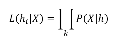
$$L(h_{i} \mid \mathbf{X}) = \prod_{k} {P(\mathbf{X}_k \mid h_{i})}$$
注意:L是未取对数前的表达式,取对数是因为概率计算很多时候假设条件独立,那么概率计算将是乘法,取对数可将乘法转为加法更方便。上面表达式中$\mathbf{X}_k$指$\mathbf{X}$取第k个值。当然,假设特征之间相互独立,也可以认为是第k个特征。
As all parameters are inside $h_i$, the gradient is a complex expression which isn't very manageable. However our goal is maximizing the likelihood, but it's easier minimizing its reciprocal:由于所有的参数都在$h_i$内,梯度是一个复杂的表达式,不是很容易处理。但是我们的目标是最大化可能性,但是最小化它的倒数会更容易:

$${max}_{i}L(h_{i} \mid \mathbf{X}) = {min}_{i} \frac {1} {L(h_{i} \mid \mathbf{X})} = {min}_{i} \frac {1} {\prod_{k} {P(\mathbf{X}_k \mid h_{i})}}$$
This can be turned into a very simple expression by applying natural logarithm (which is monotonic):取对数(对数是单调的)将得到很简单的表达式:

$${max}_{i}logL(h_{i} \mid \mathbf{X}) = {min}_{i} -logL(h_{i} \mid \mathbf{X}) = {min}_{i} \sum_{k} {-logP(\mathbf{X}_k \mid h_{i})}$$
The last term is a summation which can be easily derived and used in most of the optimization algorithms. At the end of this process, we can find a set of parameters which provides the maximum likelihood without any strong statement about prior distributions. This approach can seem very technical, but its logic is really simple and intuitive. To understand how it works, I propose a simple exercise, which is part of Gaussian mixture technique discussed also in Russel S., Norvig P., Artificial Intelligence: A Modern Approach, Pearson.最后一项是一个求和,可以很容易地使用在大多数优化算法(优化算法是找到最优参数的算法,关于优化算法请参阅wiki-Optimization algorithms)。在这个过程的最后,我们可以找到一组参数,它们提供了最大的可能性,而不需要任何关于先验分布的强声明。这种方法看起来专业,但它的逻辑非常简单和直观。为了理解它是如何工作的,我提出了一个简单的练习,这个练习是高斯混合技术的一部分。
Let's consider 100 points drawn from a Gaussian distribution with zero mean and a standard deviation equal to 2.0 (quasi-white noise made of independent samples). The plot is shown next:让我们考虑从一个均值为零、标准差为2.0的高斯分布中抽取的100个点(由独立样本构成的准白噪声)。作图如下:
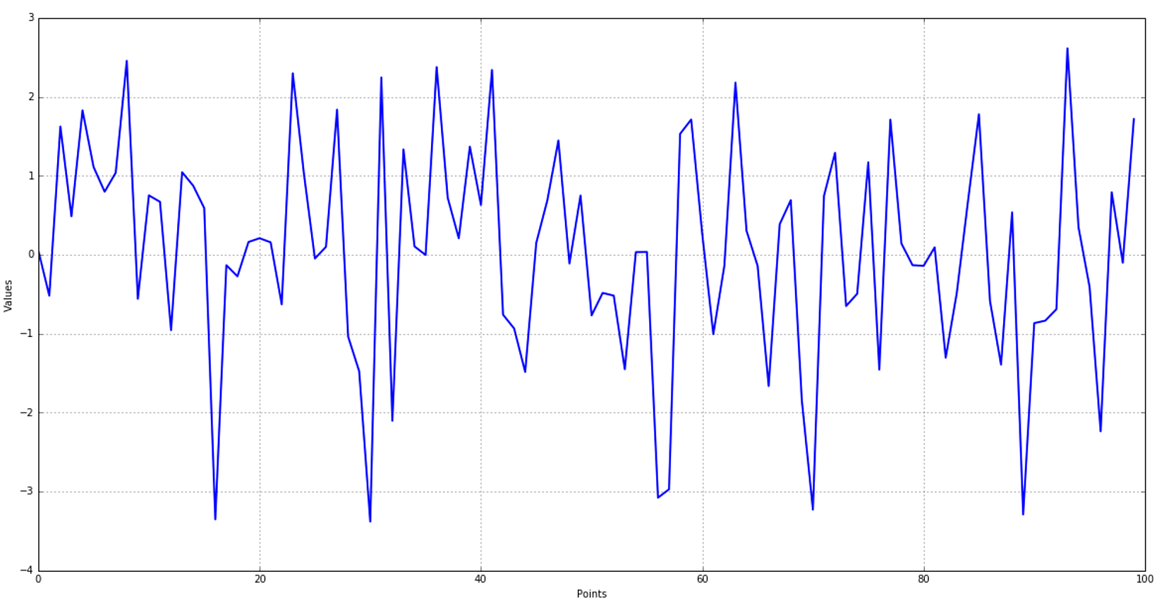 In this case, there's no need for a deep exploration (we know how they are generated), however, after restricting the hypothesis space to the Gaussian family (the most suitable considering only the graph), we'd like to find the best value for mean and variance. First of all, we need to compute the log-likelihood (which is rather simple thanks to the exponential function):在这种情况下,不需要进行深入的探索(我们知道数据是如何产生的),但是,在将假设空间限制在高斯族(考虑作图最容易)之后,我们希望找到均值和方差的最佳值(注意下式最左边其实应该是logL)。首先,我们需要计算对数似然(由于指数方程计算过程很简单):

$$logL(\mu,{\sigma}^2 \mid \mathbf{X}) = logP(\mathbf{X} \mid \mu,{\sigma}^2) = \sum_{i}{log {\frac {1} {\sqrt{2\pi{\sigma}^2}} e^{- \frac {(x_i - \mu)^2} {2{\sigma}^2 } } }}$$
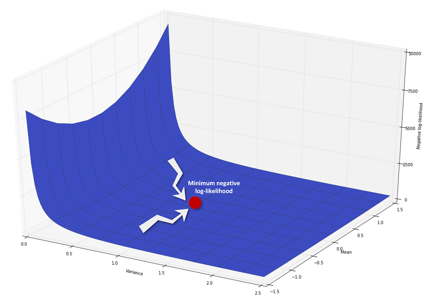
A graph of the negative log-likelihood function is plotted next. The global minimum of this function corresponds to an optimal likelihood given a certain distribution. It doesn't mean that the problem has been completely solved, because the first step of this algorithm is determining an expectation, which must be always realistic. The likelihood function, however, is quite sensitive to wrong distributions because it can easily get close to zero when the probabilities are low. For this reason, maximum-likelihood (ML) learning is often preferable to MAP learning, which needs Apriori distributions and can fail when they are not selected in the most appropriate way:接下来绘制负对数似然函数的图形。该函数的全局极小值对应于特定分布的最优似然。这并不意味着问题已经完全解决了,因为这个算法的第一步是确定一个期望,这个期望必须始终是现实的。然而,似然函数对错误的分布非常敏感,因为当概率很低时,它很容易接近于零。因此,最大似然(ML)学习通常比MAP学习更可取,MAP学习需要先验分布,如果没有以最适当的方式进行选择,则可能失败:
 This approach has been applied to a specific distribution family (which is indeed very easy to manage), but it also works perfectly when the model is more complex. Of course, it's always necessary to have an initial awareness about how the likelihood should be determined because more than one feasible family can generate the same dataset. In all these cases, Occam's razor is the best way to proceed: the simplest hypothesis should be considered first. If it doesn't fit, an extra level of complexity can be added to our model. As we'll see, in many situations, the easiest solution is the winning one, and increasing the number of parameters or using a more detailed model can only add noise and a higher possibility of overfitting.这种方法已经应用于特定的分布族(特定分布族下确实很容易处理),但是当模型更复杂时,它也能很好地工作。当然,总是有必要对如何确定似然有一个初步的认识,因为多个可行的族可以生成相同的数据集。在所有这些情况下,奥卡姆剃刀是最好的方法:即首先应该考虑最简单的假设。如果它不适合,我们的模型可以增加额外的复杂性。正如我们将看到的,在许多情况下,最简单的解决方案是获胜的方案,增加参数的数量或使用更详细的模型只会增加噪音和过度拟合的可能性。
2.4 Elements of information theory信息理论因素
A machine learning problem can also be analyzed in terms of information transfer or exchange. Our dataset is composed of n features, which are considered independent (for simplicity, even if it's often a realistic assumption) drawn from n different statistical distributions. Therefore, there are n probability density functions $p_i (x)$ which must be approximated through other n $q_i (x)$ functions. In any machine learning task, it's very important to understand how two corresponding distributions diverge and what is the amount of information we lose when approximating the original dataset.机器学习问题也可以从信息传递或交换的角度进行分析。我们的数据集是由n个特征组成的,它们被认为是独立的(为了简单起见,即使这通常是一个现实的假设),这些特征来自于n个不同的统计分布。因此,有n个概率密度函数$p_i (x)$必须通过其他n个$q_i (x)$函数逼近。在任何机器学习任务中,理解两个对应的分布是如何偏离的以及在接近原始数据集时我们丢失了多少信息量是非常重要的。
【 这里补充信息量的概念。 首先是信息量。假设我们听到了两件事,分别如下:
- 事件A:巴西队进入了2018世界杯决赛圈。
- 事件B:中国队进入了2018世界杯决赛圈。
仅凭直觉来说,显而易见事件B的信息量比事件A的信息量要大。究其原因,是因为事件A发生的概率很大,事件B发生的概率很小。所以当越不可能的事件发生了,我们获取到的信息量就越大。越可能发生的事件发生了,我们获取到的信息量就越小。那么信息量应该和事件发生的概率有关。
假设X是一个离散型随机变量,其取值集合为$\chi$,概率分布函数$p(x)=Pr(X=x),x∈\chi$,则定义事件$X=x_0$的信息量为:
$$I(x_0)=-log(p(x_0))$$
概率为1的事件发生毫无信息量,概率为0时间发生无穷信息量,概率大的事件发生的信息量小于概率小的事件发生的信息量。所以信息量定义的函数需要单调递减且f(0)=∞、f(1)=0。
熵其实是信息量的期望。 】
The most useful measure is called entropy:最有用的测量叫做熵:

$$H(X)=-\sum_{x \in X}{p(x)\log p(x)}$$
This value is proportional to the uncertainty of X and it's measured in bits (if the logarithm has another base, this unit can change too). For many purposes, a high entropy is preferable, because it means that a certain feature contains more information. For example, in tossing a coin (two possible outcomes), H(X) = 1 bit, but if the number of outcomes grows, even with the same probability, H(X) also does because of a higher number of different values and therefore increased variability. It's possible to prove that for a Gaussian distribution (using natural logarithm):熵值与X的不确定性成正比(作者这里的意思是用熵来代表不确定度。但请注意,熵不涉及变量的大小,甚至,比如变量是分类的时候,变量可以用非数值表示,此时方差不存在,那么谈不上熵与方差有什么关系。比如:等可能取红球和黑球,那么p(红球)=p(黑球)=0.5,那么对数底取2时熵为1,此时并没有什么方差。即使分类变量有确定的数值表示形式,也不一定熵高者方差大。比如,等可能取整数1到9,那么方差为20/3,对数底取2时熵为9ln9;等可能取整数1、9,那么方差为16,熵为2ln2;等可能取整数1到3,那么方差为2/3,熵为3ln3。对于连续变量,若服从高斯分布,那么,方差大者熵大,熵大者方差也大。),它是以位来度量的(也可采用其他单位来度量,取决于以什么为对数底了,比方也可以e为底)。在很多情况下,高熵是可取的,因为它意味着某个特性包含更多的信息。例如,在抛硬币(两种可能的结果)时,H(X)=1位,但是如果结果的数量增加了,即使概率相同,H(X)也会增加,因为不同值的数量增加了,因此变异性也增加了(抛硬币不是合适的例子,况且,抛硬币例子结果只有正面、反面、竖起来,结果数量最大为3,结果数量从2变为3概率不可能相同。我举一个更恰当的例子吧。情况1, X等可能取-1、1;情况2,Y等可能取自然数-4到4。那么H(X)=1、H(Y)=3。这里,结果数量越多(变异越大),则熵越大。)。(用自然对数)可以证明对高斯分布有:
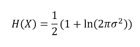
$$H(X)=\frac {1}{2}(1+\ln{(2\pi{\sigma}^2)})$$
【
高斯分布熵与方差关系之证明:
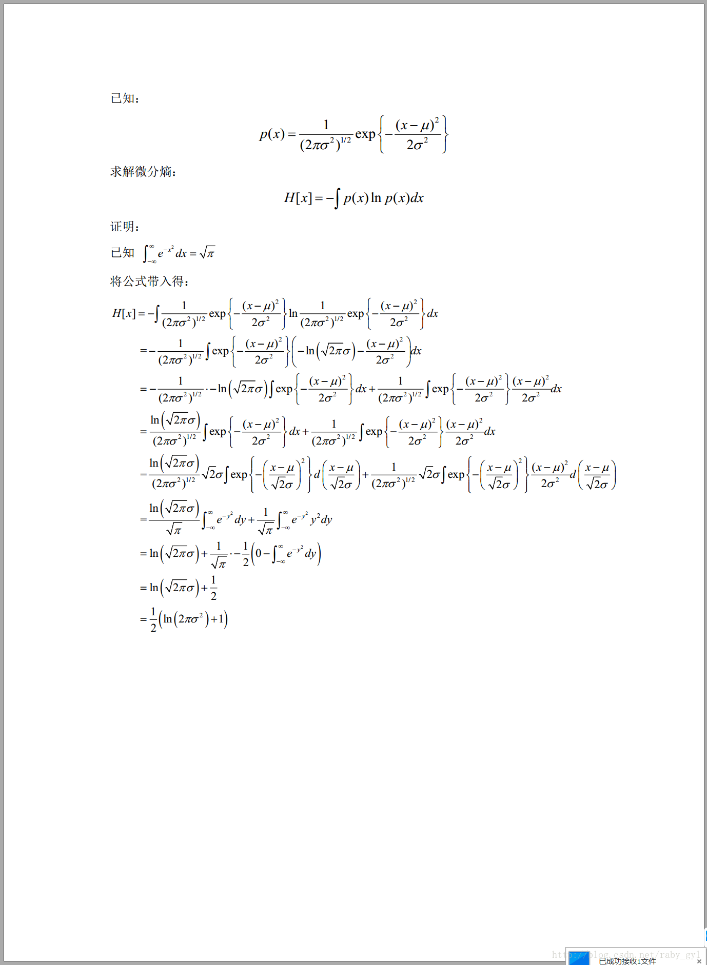
$$p(x)=\frac {1} {\sqrt{2\pi{\sigma}^2}} e^{- \frac {(x_i - \mu)^2} {2{\sigma}^2}}$$
$$\int_{-\infty}^{+\infty} { e^{-x^2}} \ dx = \sqrt{\pi}$$
$$\begin{align}
H(X) & = -\int { p(x)\ln p(x)} \ dx \\
& = -\int { \frac {1} {\sqrt{2\pi{\sigma}^2}} e^{- \frac {(x - \mu)^2} {2{\sigma}^2}}\ln {\frac {1} {\sqrt{2\pi{\sigma}^2}} e^{- \frac {(x - \mu)^2} {2{\sigma}^2}}}} \ dx \\
& = -\frac {1} {\sqrt{2\pi{\sigma}^2}}\int { e^{- \frac {(x - \mu)^2} {2{\sigma}^2}}\ln {\frac {1}{\sqrt{2\pi{\sigma}^2}} e^{- \frac {(x - \mu)^2} {2{\sigma}^2}}}} \ dx \\
& =  \frac {\ln {\sqrt{2\pi{\sigma}^2}}} {\sqrt{2\pi{\sigma}^2}} \int {e^{- \frac {(x - \mu)^2} {2{\sigma}^2}}} \ dx + \frac {1} {\sqrt{2\pi{\sigma}^2}}\int { \frac {(x - \mu)^2} {2{\sigma}^2} e^{-\frac {(x - \mu)^2} {2{\sigma}^2}}} \ dx \\
& =  \frac {\ln {\sqrt{2\pi{\sigma}^2}}} {\sqrt{2\pi{\sigma}^2}} \int {e^{- y^2}} \ d(\sqrt{2}\sigma y + \mu) + \frac {1} {\sqrt{2\pi{\sigma}^2}}\int { y^2 e^{-y^2}} \ d(\sqrt{2}\sigma y + \mu) \\
& =  \frac {\ln {\sqrt{2\pi{\sigma}^2}}} {\sqrt{\pi}} \int_{-\infty}^{+\infty} {e^{- y^2}} \ dy + \frac {1} {\sqrt{\pi}} \int_{-\infty}^{+\infty} { y^2 e^{-y^2}} \ dy \\
& =  \ln {\sqrt{2\pi{\sigma}^2}} + \frac {1} {\sqrt{\pi}} \int_{-\infty}^{+\infty} { -\frac{1}{2} y } \ d(e^{-y^2}) \\
& =  \ln {\sqrt{2\pi{\sigma}^2}} + \frac {1} {\sqrt{\pi}}(-\frac{1}{2}) \int_{-\infty}^{+\infty} {  y } \ d(e^{-y^2}) \\
& =  \ln {\sqrt{2\pi{\sigma}^2}} + \frac {1} {\sqrt{\pi}}(-\frac{1}{2})(\left. ye^{-y^2} \right|_{-\infty}^{+\infty} - \int_{-\infty}^{+\infty} {e^{-y^2}} \ dy) \\
& =  \ln {\sqrt{2\pi{\sigma}^2}} + \frac {1} {\sqrt{\pi}}(-\frac{1}{2})(0 - \sqrt{\pi}) \\
& =  \frac {1}{2}(1+\ln{(2\pi{\sigma}^2)})
\end{align}$$
用到了分部积分知识。
】
【 对于经验分布,证明方差大者熵大:可证明方差增大时熵增大,以证明方差大者熵大。 】
【
注意:
1、熵只依赖于随机变量的分布,与随机变量取值无关,所以也可以将X的熵记作H(p)。
2、令0log0=0(因为某个取值概率可能为0)。
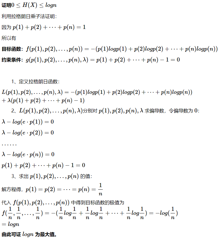
3、对于离散型随机变量,随机变量的取值个数越多,状态数也就越多,信息熵就越大,混乱程度就越大。当随机分布为均匀分布时,熵最大,且0≤H(X)≤logn。(P(X)在0到1之间那么显然熵大于等于0,当X只有一个取值时,熵取最小值0;熵小于等于$\log n$,当均匀分布时熵取最大值$\log n$(可用拉格朗日乘子法证明https://www.cnblogs.com/kyrieng/p/8694705.html )。)
 4、对于连续性随机变量,熵等于概率密度与对数概率密度的乘积的积分。
】
So, the entropy is proportional to the variance, which is a measure of the amount of information carried by a single feature. In the next chapter, we're going to discuss a method for feature selection based on variance threshold. Gaussian distributions are very common, so this example can be considered just as a general approach to feature filtering: low variance implies low information level and a model could often discard all those features.所以,(对于高斯分布,)熵与方差成正比,方差是衡量单个特征携带的信息量的一个指标。在下一章中,我们将讨论一种基于方差阈值的特征选择方法。高斯分布是非常常见的,所以这个例子可以看作是一种特征过滤的通用方法:低方差意味着低信息水平,一个模型常常会丢弃所有这些特征(即低方差低信息水平的特征)。
对于服从高斯分布的特征,自然有充足理由根据方差选择特征,因为高斯分布方差大者信息量高。连续变量或多或少均近似高斯分布。那么对于含有计数count特征、分类特征的数据是否可以根据特征方差大小选择特征呢?。这仍然是一个需要深究的话题。留待时间充裕再深究吧!!!! 可以肯定的是,可以根据特征的熵选择特征。无论是连续变量特征、计数特征、和分类特征,根据数据集计算熵都是很方便的(连续特征体现在数据集上仍是离散的,某个指标,获取数据阶段精度不可能无限。),熵更大的特征更重要。
In the following figure, there's a plot of H(X) for a Gaussian distribution expressed in nats (which is the corresponding unit measure when using natural logarithms):下图是高斯分布的H(X)曲线,以nats表示(这是使用自然对数时的对应单位度量):
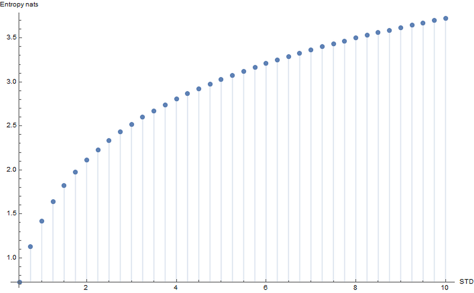 For example, if a dataset is made up of some features whose variance (here it's more convenient talking about standard deviation) is bounded between 8 and 10 and a few with STD < 1.5, the latter could be discarded with a limited loss in terms of information. These concepts are very important in real-life problems when large datasets must be cleaned and processed in an efficient way.例如,如果一个数据集是由一些特征组成的,这些特征的方差(在这里讨论标准差更方便)在8到10之间,一些STD < 1.5,后者可以被丢弃,信息损失有限。信息熵概念对大数据集很重要,大数据集必须有效清洗处理。
用信息理论怎么理解特征缩放呢,很多算法要求特征缩放,显然这将混淆各特征的信息量? 我是这么理解的,暂时不知道这个理解正确与否。基于协方差矩阵过滤特征(如PCA)是采用信息理论选取特征;也可以根据模型(或者说根据目标变量)来确定特征信息含量比例(确定每个特征对应的参数),有些算法需要对特征进行缩放,有些也不一定要缩放,但无论如何,缩放没有坏处,将改善条件数,使算法加速收敛。缩放后的特征具有相同的方差,这等于放弃未见目标变量前的先入为主信息。各特征对目标变量的信息贡献比例由缩放比例和算法中特征对应的参数共同决定。
If we have a target probability distribution p(x), which is approximated by another distribution q(x), a useful measure is cross-entropy between p and q (we are using the discrete definition as our problems must be solved using numerical computations):如果我们有一个目标概率分布p(x),用另一个分布q(x)近似,一个有用的度量是p和q之间的交叉熵(我们使用离散定义,因为我们的问题必须用数值计算来解决):

$$H(P,Q) = -\sum_{x \in X}{p(x)log_2q(x)}$$
If the logarithm base is 2, it measures the number of bits requested to decode an event drawn from P when using a code optimized for Q. In many machine learning problems, we have a source distribution and we need to train an estimator to be able to identify correctly the class of a sample. If the error is null, P = Q and the cross-entropy is minimum (corresponding to the entropy H(P)). However, as a null error is almost impossible when working with Q, we need to pay a price of H(P, Q) bits, to determine the right class starting from a prediction. Our goal is often to minimize it, so to reduce this price under a threshold that cannot alter the predicted output if not paid. In other words, think about a binary output and a sigmoid function: we have a threshold of 0.5 (this is the maximum price we can pay) to identify the correct class using a step function (0.6 -> 1, 0.1 -> 0, 0.4999 -> 0, and so on). As we're not able to pay this price, since our classifier doesn't know the original distribution, it's necessary to reduce the cross-entropy under a tolerable noise-robustness threshold (which is always the smallest achievable one).如果以2为底的对数,上式测量的是用Q解码取自P的事件的位数。在许多机器学习问题中,我们有一个源分布,我们需要训练估计器来正确地识别样本的类。若误差是零,那P=Q且交叉熵最小(即等于熵H(P))。然而,当使用Q时零错误几乎是不可能的,我们需要付出H(P,Q)位的代价,以预测确定正确的类。我们的目标通常是最小化交叉熵H(P,Q),以减少代价到特定阈值,如不付出这个代价就不能得到预测输出。换句话说,设想二分类输出和sigmoid函数:我们有一个0.5的阈值(这是我们可以支付的最大代价),使用一个步骤函数(0.6-> 1、0.1->0、0.4999->0等等)来识别正确的分类。由于我们无法支付这个代价,既然分类器不知道原始分布,所以有必要在一个可容忍的噪声-鲁棒性阈值(通常是最小可实现的阈值)下降低交叉熵。
【 为什么交叉熵足够小Q就可很好描述P?
3 相对熵(KL散度)
相对熵又称KL散度,如果我们对于同一个随机变量X有两个单独的概率分布P(X)和Q(X),我们可以使用KL散度(Kullback-Leibler (KL) divergence)来衡量这两个分布的差异。
wiki对相对熵的定义:
> In the context of machine learning, $D_{KL} (P‖Q)$ is often called the information gain achieved if P is used instead of Q.
即如果用P而不是用Q来描述问题,得到的信息增益。
在机器学习中,假设P表示实际分布,比如[1,0,0]表示当前样本属于第一类。Q用来表示模型所预测的分布,比如[0.6,0.2,0.2]。
显然,如果用P来描述样本,那非常完美。而用Q来描述,虽可大致描述,但是不是那么的完美,信息量不足,需要额外的一些“信息增益”才能达到和P一样完美的描述。如果我们的Q通过反复训练,也能完美的描述样本,那么就不再需要额外的“信息增量”,Q等价于P。
KL散度的计算公式:
$$D_{KL}(P||Q) = \sum_{x \in X}{p(x)log{\frac{p(x)}{q(x)}}} = E_{p(x)}{\frac{p(x)}{q(x)}}$$
性质: 1、如果p(x)和q(x)两个分布相同,那么相对熵等于0
2、$D_{KL} (P‖Q) \ne D_{KL} (Q‖P)$,相对熵具有不对称性。大家可以举个简单例子算一下。
3、$D_{KL} (P‖Q)\ge 0$证明如下(利用Jensen不等式https://en.wikipedia.org/wiki/Jensen%27s_inequality) :
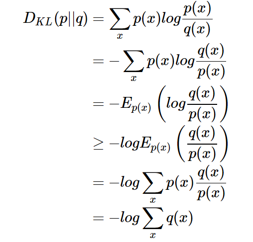 而概率和为1即
$\sum{p(x_i)}=1$,证毕。
4、$D_{KL} (P‖Q)=H(P,Q)-H(P)$,KL散度=交叉熵-实际分布的熵。实际分布的熵是正的常数,交叉熵和KL散度是变量,那么当P=Q时交叉熵和KL散度同时取得最小值。
由性质4可知:交叉熵足够小Q就可很好描述P。 】
In order to understand how a machine learning approach is performing, it's also useful to introduce a conditional entropy or the uncertainty of Y given the knowledge of X:为理解机器学习方法的表现,引入条件熵(或称之为已知X时Y的不确定性)很有用:
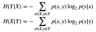
$$H(Y|X)=-\sum_{x \in X, y \in Y}{p(x,y)\log_2 {p(y|x)}}$$
$$H(X|Y)=-\sum_{x \in X, y \in Y}{p(x,y)\log_2 {p(x|y)}}$$
【
条件熵H(Y|X)表示在已知随机变量X的条件下随机变量Y的不确定性。条件熵H(Y|X)定义为X给定条件下Y的条件概率分布的熵对X的数学期望:
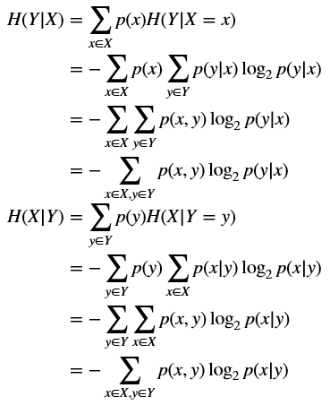
$$
\begin{align}
H(Y|X)  &=\sum_{x \in X}{p(x)H(Y|X=x)}  \\
&   =-\sum_{x \in X}{p(x)\sum_{y \in Y}{p(y|x)\log_2 {p(y|x)}}}  \\
&   =-\sum_{x \in X}{\sum_{y \in Y}{p(x,y)\log_2 {p(y|x)}}}  \\
&   =-\sum_{x \in X,y \in Y}{p(x,y)\log_2 {p(y|x)}}  \\
\end{align}
$$
$$
\begin{align}
H(X|Y)  &=\sum_{y \in Y}{p(y)H(X|Y=y)}  \\
&   =-\sum_{y \in Y}{p(y)\sum_{x \in X}{p(x|y)\log_2 {p(x|y)}}}  \\
&   =-\sum_{y \in Y}{\sum_{x \in X}{p(x,y)\log_2 {p(x|y)}}}  \\
&   =-\sum_{x \in X,y \in Y}{p(x,y)\log_2 {p(x|y)}}  \\
\end{align}
$$
联合熵、条件熵、边际熵关系:

$$H(X;Y)=H(Y|X)+H(X)=H(X|Y)+H(Y)$$
联合熵、条件熵、边际熵关系之证明:
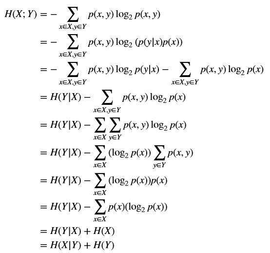
$$
\begin{align}
H(X;Y)  &=-\sum_{x \in X, y \in Y}{p(x,y)\log_2 {p(x,y)}}   \\
&   =-\sum_{x \in X, y \in Y}{p(x,y)\log_2 {(p(y|x)p(x))}}  \\
&   =-\sum_{x \in X, y \in Y}{p(x,y)\log_2 {p(y|x)}}-\sum_{x \in X, y \in Y}{p(x,y)\log_2 {p(x)}}   \\
&   =H(Y|X)-\sum_{x \in X, y \in Y}{p(x,y)\log_2 {p(x)}}    \\
&   =H(Y|X)-\sum_{x \in X}{\sum_{y \in Y}{p(x,y)\log_2 {p(x)}}}  \\
&   =H(Y|X)-\sum_{x \in X}{(\log_2 {p(x))}\sum_{y \in Y}{p(x,y)}}  \\
&   =H(Y|X)-\sum_{x \in X}{(\log_2 p(x))p(x)}  \\
&   =H(Y|X)-\sum_{x \in X}{p(x)(\log_2 p(x))}  \\
&   =H(Y|X)+H(X)  \\
&   =H(X|Y)+H(Y)   \\
\end{align}
$$
】
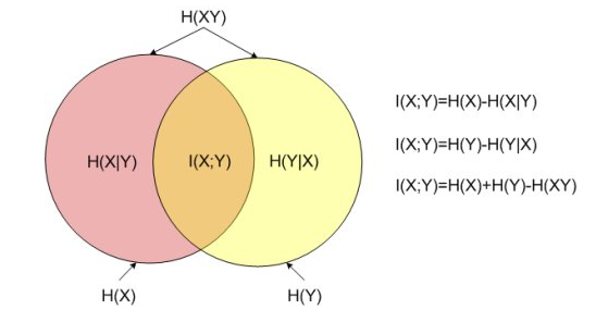
Through this concept, it's possible to introduce the idea of mutual information I(X;Y), which is the amount of information shared by both variables and therefore, the reduction of uncertainty about Y provided by the knowledge of X:通过这个概念,可以引入互信息I(X;Y)的概念,这是两个变量共享的信息量,即,Y的不确定减去已知X时Y的不确定性:

$$I(X;Y)=H(Y)-H(Y|X)=H(X)-H(X|Y)$$
【
互信息的定义:
在概率论和信息论中,两个随机变量的互信息(Mutual Information,简称MI)或转移信息(transinformation)是变量间相互依赖性的量度。

$$I(X;Y)=\sum_{x \in X, y \in Y}{p(x,y)\log_2 {(\frac{p(x,y)}{p(x)p(y)})}}$$
互信息、边际熵、条件熵关系的证明:
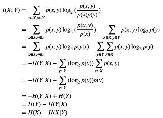
$$
\begin{align}
I(X;Y)  &=\sum_{x \in X, y \in Y}{p(x,y)\log_2 {(\frac{p(x,y)}{p(x)p(y)})}} \\
&   =\sum_{x \in X, y \in Y}{p(x,y)\log_2 {(\frac{p(x,y)}{p(x)})}}-\sum_{x \in X, y \in Y}{p(x,y)\log_2 {p(y)}} \\
&   =\sum_{x \in X, y \in Y}{p(x,y)\log_2 {p(y|x)}}-\sum_{y \in Y}{\sum_{x \in X}{p(x,y)\log_2 {p(y)}}} \\
&   =-H(Y|X)-\sum_{y \in Y}{(\log_2 {p(y)})\sum_{x \in X}{p(x,y)}}   \\
&   =-H(Y|X)-\sum_{y \in Y}{(\log_2 {p(y)})p(y)}   \\
&   =-H(Y|X)+H(Y)   \\
&   =H(Y)-H(Y|X)   \\
&   =H(X)-H(X|Y)   \\
\end{align}
$$
联合熵与互信息之和等于边际熵之和:

$$H(X;Y)+I(X;Y)=H(Y|X)+H(X)+H(Y)-H(Y|X)=H(X)+H(Y)$$
边际熵、条件熵、联合熵、互信息之间关系示意图:
 】
】
Intuitively, when X and Y are independent, they don't share any information. However, in machine learning tasks, there's a very tight dependence between an original feature and its prediction, so we want to maximize the information shared by both distributions. If the conditional entropy is small enough (so X is able to describe Y quite well), the mutual information gets close to the marginal entropy H(X), which measures the amount of information we want to learn.直觉上,若X与Y独立,它们之间不共享任何信息。然而,在机器学习任务中,一个原始特性和它的预测之间有非常紧密的依赖关系,所以我们想要最大化两个分布共享的信息。如果条件熵足够小(因此X可以很好地描述Y),互信息就会接近边际熵H(Y),边际熵H(Y)衡量我们想要学习的信息量。
【 为什么条件熵足够小X就可很好描述Y? 答:对于特定机器学习问题,数据集确定,那么X和Y的熵即边际熵一定。条件熵足够小,那么互信息足够大,那么X与Y紧密依赖,那么X可以很好地描述Y。 】
An interesting learning approach based on the information theory, called Minimum Description Length (MDL), is discussed in Russel S., Norvig P., Artificial Intelligence: A Modern Approach, Pearson, where I suggest you look for any further information about these topics.最小化描述长度(MDL)是基于信息理论的一个有趣学习方法。
datetime:2018/11/16 22:51
2.5 References参考文献
2.6 Summary总结
3 Feature Selection and Feature Engineering特征选择与特征工程
3.1 scikit-learn toy datasets scikit-learn玩具数据集
3.2 Creating training and test sets建立训练测试集
In the following figure, there's a schematic representation of process that split datasets into training and test sets:在下面的图中,有划分训练、测试集过程的示意图:
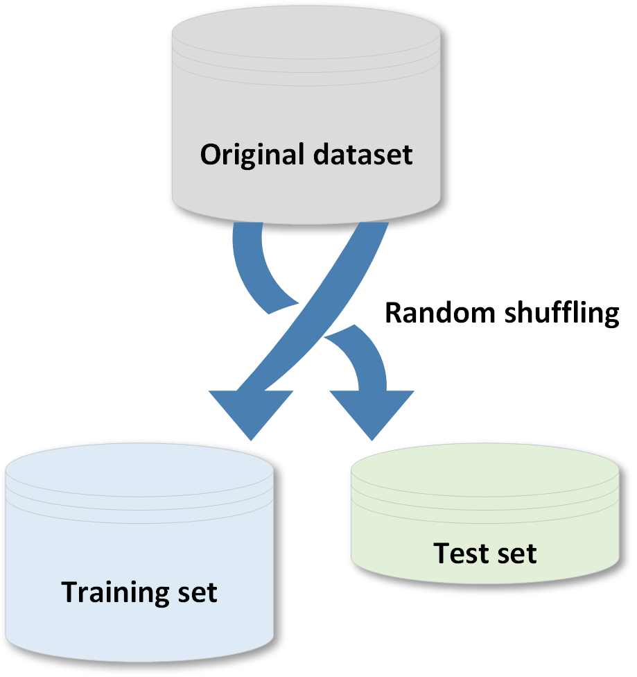 There are two main rules in performing such an operation:进行这一操作的两条主要规则:
- Both datasets must reflect the original distribution训练、测试集均应反映原始分布
- The original dataset must be randomly shuffled before the split phase in order to avoid a correlation between consequent elements为了避免后续元素之间的相关性,在分离阶段之前必须随机打乱原始数据集
3.3 Managing categorical data处理分类数据
Categorical target variables representing by progressive integer number have drawback: all labels are turned into sequential numbers. A classifier which works with real values will then consider similar numbers according to their distance, without any concern for semantics. For this reason, it's often preferable to use so-called one-hot encoding。用累进整数表示的分类目标变量有缺点:所有的标签都变成了连续数字。使用实值的分类器将根据距离考虑相似的数字,而不考虑语义。因此,最好使用独热编码。
对于分类特征呢?按Feature_Engineering_for_Machine_Learning,特征中的分类变量也最好不要停留在累进整数。当然,需要考虑计算消耗。
3.4 Managing missing features处理缺失特征
Sometimes a dataset can contain missing features, so there are a few options that can be taken into account:有时一个数据集可能包含缺失的特性,因此有一些选项可以考虑:
- Removing the whole line去掉整行
- Creating sub-model to predict those features创建子模型来预测这些(缺失值)特征
- Using an automatic strategy to input them according to the other known values根据其他已知值自动补全
The first option is the most drastic one and should be considered only when the dataset is quite large, the number of missing features is high, and any prediction could be risky. The second option is much more difficult because it's necessary to determine a supervised strategy to train a model for each feature and, finally, to predict their value. Considering all pros and cons, the third option is likely to be the best choice.第一个选择是最激烈的,只有当数据集相当大,缺失特性个数很多,任何预测都可能有风险时才应该考虑。 第二种选择要困难得多,因为有必要确定一种监督策略来训练每个特性的模型,并最终预测它们的值。考虑全部优缺点,第三种很可能是最优选择。
3.5 Data scaling and normalization数据缩放与正态化
In the following figure, there's a comparison between a raw dataset and the same dataset scaled and centered:在下面的图中,将原始数据集和相同数据集经缩放并中心化进行比较:
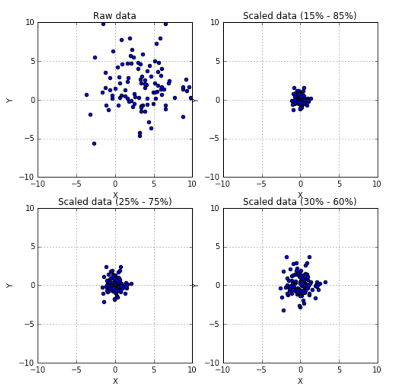
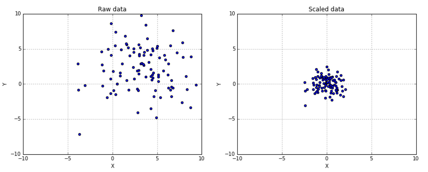 If you need a more powerful scaling feature, with a superior control on outliers and the possibility to select a quantile range, there's also the class RobustScaler.如果你需要一个更强大的缩放功能,对离群值有更好的控制并可选择分位数范围,那可以用
RobustScaler。
The results are shown in the following figures:结果如下图所示:
 scikit-learn also provides a class for per-sample normalization,
 Normalizer. It can apply max, l1 and l2 norms to each element of a dataset. scikit-learn还提供了一个类,用于对每个样本进行规范化,即Normalizer。它可以对数据集的每个元素应用max(除以特征列的最大值)、l1(除以特征列的l1范数)和l2(除以特征列的l1范数)规范。
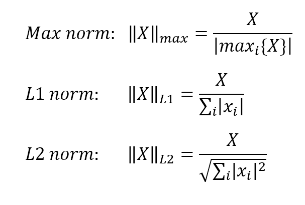
$$Max \ norm:{||X||}_{max}=\frac{X}{|max_{i} {\{X\}}|}$$
$$L1 \ norm:{||X||}_{L1}=\frac{X}{\sum_{i}{|X|}}$$
$$L2 \ norm:{||X||}_{L2}=\frac{X} {\sqrt{\sum_{i}{|X|^2}}}$$
3.6 Feature selection and filtering特征选择与过滤
An unnormalized dataset with many features contains information proportional to the independence of all features and their variance. Let's consider a small dataset with three features, generated with random Gaussian distributions:具有许多特征的非规范化数据集包含与所有特征的独立性及其方差成比例的信息。考虑一个具有三个特性的小数据集,它是用随机高斯分布生成的:
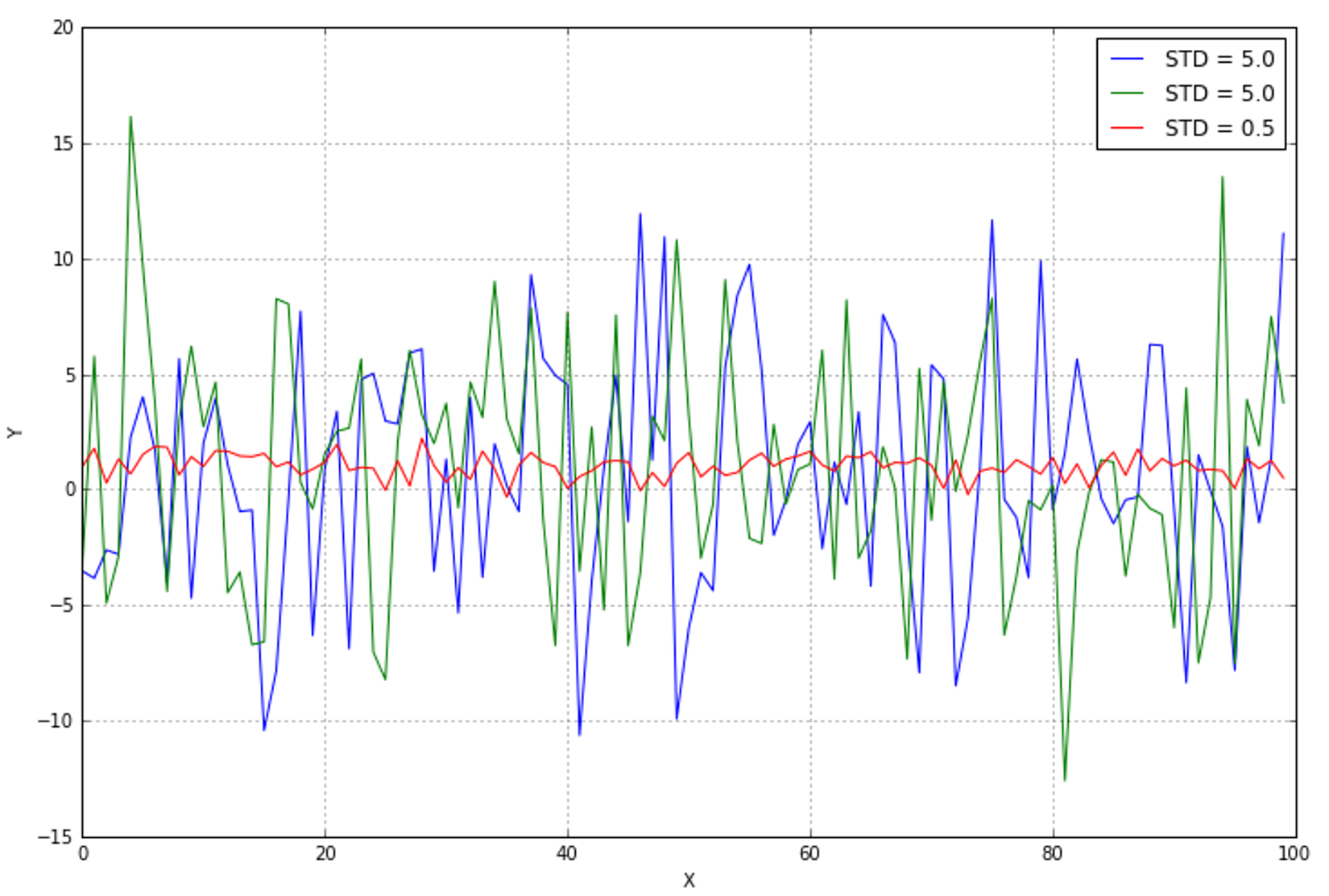 Even without further analysis, it's obvious that the central line (with the lowest variance) is almost constant and doesn't provide any useful information. If you remember the previous chapter, the entropy H(X) is quite small, while the other two variables carry more information. A variance threshold is, therefore, a useful approach to remove all those elements whose contribution (in terms of variability and so, information) is under a predefined level. scikit-learn provides the class
 VarianceThreshold that can easily solve this problem. By applying it on the previous dataset, we get the following result:
Let's consider the following figure (without any particular interpretation):即使没有进一步的分析,很明显,中心那条线(方差最小的)几乎是恒定的,并且没有提供任何有用的信息。方差小意味着熵H(X)很小,而其他两变量含有更多信息。因此,方差阈值是一种有用的方法,可以删除所有那些贡献(就可变性和信息而言)在预定义级别之下的元素。scikit-learn提供VarianceThreshold类可以容易解决这一问题。
There are also many univariate methods that can be used in order to select the best features according to specific criteria based on F-tests and p-values, such as chi-square or ANOVA. However, their discussion is beyond the scope of this book and the reader can find further information in Freedman D., Pisani R., Purves R., Statistics, Norton & Company.也有许多单变量方法可以用来根据基于F检验和p值的特定标准来选择最佳特征,例如卡方或方差分析。已超本书的该讨论的范围。
搞清楚chi-square和ANOVA特征选择详情,并属于特征选择书本中2.6的哪类。
【 卡方检验与特征选择:
- 简介
卡方检验是一种用途非常广泛的假设检验方法,在统计推断中使用非常多,可以检测多个分类变量之间的相关性是否显著。
- 基本原理
卡方检验就是统计样本的实际观测值和理论推断值之间的偏离程度,如果chi-square值越大,二者偏差程度越大;反之,二者偏差越小。若chi-square为0,表明理论和实际值完全符合。
- 原型
1) 提出假设
H0: 总体X的分布律为$P(X= x_i )=p_i ,i=1,2,\ldots $
2)将总体X的取值范围分成k个互不相交的小区间A1,A2,A3,…,Ak,如可取:
A1=(a0,a1],A2=(a1,a2],...,Ak=(ak-1,ak),
其中:
i. a0可取$-\infty$,ak可取$+\infty$,区间的划分视具体情况而定
ii. 每个小区间所含的样本值个数不小于5
iii. 区间个数k适中
3)把落入第i个小区间的Ai的样本值的个数记作fi, 所有组频数之和f1+f2+...+fk等于样本容量n。
4)当H0为真时,根据所假设的总体理论分布,可算出总体X的值落入第i 个小区间Ai的概率pi,于是,npi就是落入第i个小区间Ai的样本值的理论频数(理论值)。
5)当H0为真时,n次试验中样本值落入第i个小区间Ai的频率fi/n与概率pi应很接近,当H0不真时,则fi/n与pi相差很大。
6)基于上面想法,引入下面统计量:
$${\chi}^2 = \sum_{i=1}^{k} {(f_i-n p_i)^2/(n p_i)}$$
,便得到了在H0假设成立的情况下服从自由度为k-1的卡方分布。
- 四表格法 四表格法是一种检验方法,主要检测两个分类变量X和Y,他们的值域分别为{x1, x2}和{y1, y2},其样本频数列联表为:
| y1 | y2 | 总计 | |
|---|---|---|---|
| x1 | a | b | a+b |
| x2 | c | d | c+d |
| 总计 | a+c | b+d | a+b+c+d |
按照上面原型: 1) 提出假设H0:X与Y有关系 2)计算chi-square值, chi-square值越大说明X与Y偏离程度越大,X与Y就相关性就越小,也就是越不相关。
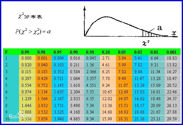
可以查阅下表,来确定X与Y是否有关系的可信度:
 在上表中:
i. F代表自由度, 在表格中自由度v=(行数-1)(列数-1) ,所以四表格中,行数=列数=2,所以四表格中自由度v=1
ii. 显著水平α为第一行绿色部分。代表的二者的相关程度
iii. 从第二行,第二列起,每个值代表计算出来的chi-square值。
举例当F=1时, P(chi > 6.64) = 0.01 , 表示当chi方值>6.64的时候,相关的概率为0.01. 也就是相关的可信度是0.01。 不相关的可信度是0.99
- 举例:
| 男 | 女 | 总计 | |
|---|---|---|---|
| 化妆 | 15(55) | 95(55) | 110 |
| 不化妆 | 85(45) | 5(45) | 90 |
| 总计 | 100 | 100 | 200 |
其中,每个格子的数是按假设计算得来的,这里我们假设H0:X(化妆与否)与Y(性别)不相关,那按这种假设化妆男、化妆女、不化妆男、不化妆女应该为55、55、45、45。
那么卡方=(15-55)^2/55 + (95-55)^2/55 + (85-45)^2/45 + (5-45)^2/45 = 129.30 自由度=(2-1)(2-1)=1,所以p(chi_square>129.30)远小于0.001(自由度1、卡方为129.30对应的显著性水平显然远小于0.001),H0是不能接受的,因此X与Y有很强的相关性。
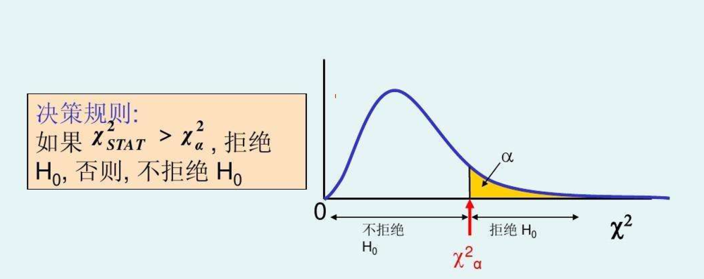
卡方检验接受假设或拒绝假设的示意图:
 datetime: 2018/11/18 0:58
卡方检验与特征选择: 假设我们有x1到xn共n个特征和目标y,分别检验每个特征与目标的相关性,特征选择可保留相关性大者(不相关假设的显著水平低者)。 显然,机器学习的特征工程中将会把这种特征选择归入特征过滤。 】
【 ANOVA与特征选择: 百度百科垃圾,又要自己翻译wiki了Analysis of variance。有空再说。 https://www.cnblogs.com/stevenlk/p/6543628.html 这个博客不错。 】
3.7 Principal component analysis主成分分析(PCA)
In general, if we consider a Euclidean space, we have:考虑欧式空间,有:

$$\mathbf{X}=\{\vec{x_1},\vec{x_2},\ldots,\vec{x_n}\} \ where \ \vec{x_n} \in \mathbb{R}^m \ and \ \vec{x_i}=x_{i1}\vec{e_1}+x_{i2}\vec{e_2}+\dots+x_{im}\vec{e_m}$$
So each point is expressed using an orthonormal basis made of m linearly independent vectors. Let's consider the following figure (without any particular interpretation):所以每个点都是由m个线性无关的向量组成的标准正交基表示的。让我们考虑下面的图(没有任何特别的解释):
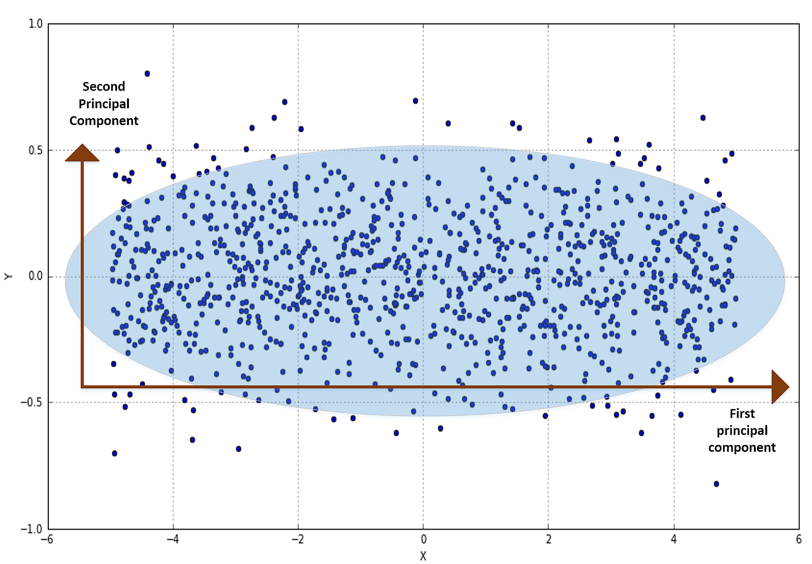 It doesn't matter which distributions generated X=(x1,x2), however, the variance of the horizontal component is clearly higher than the vertical one. (x1,x2)的分布并不重要,但水平成分的方差明显高于垂直成分。
In order to assess how much information is brought by each component, and the correlation among them, a useful tool is the covariance matrix (if the dataset has zero mean, we can use the correlation matrix):为了评估每个组件带来了多少信息,以及它们之间的相关性,一个有用的工具是协方差矩阵(如果数据集的均值为零,我们可以使用相关矩阵):
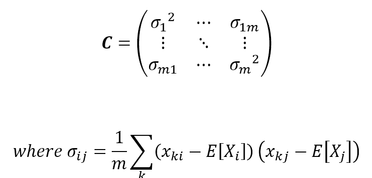
$$\mathbf{C}=\begin{pmatrix} {{\sigma}_1}^2 & \cdots & {\sigma}_{1m} \\ \vdots & \ddots & \vdots \\ {\sigma}_{m1} & \cdots & {{\sigma}_m}^2  \end{pmatrix} \\
where \ {\sigma}_{ij}=\frac{1}{m}\sum_{k}{(x_{ki}-E[X_i])(x_{kj}-E[X_j])}$$
C is symmetric and positive semidefinite, so all the eigenvalues are non-negative, but what's the meaning of each value? The covariance matrix for the previous example is:C是对称的半正定的,所以所有的特征值都是非负的,但是每个值的意义是什么呢?上一个例子的协方差矩阵是:
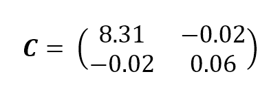
$$\mathbf{C}=\begin{pmatrix} 8.31 & -0.02 \\ -0.02 & 0.06 \end{pmatrix}$$
As expected, the horizontal variance is quite a bit higher than the vertical one. Moreover, the other values are close to zero. If you remember the definition and, for simplicity, remove the mean term, they represent the cross-correlation between couples of components. It's obvious that in our example, x1 and x2 are uncorrelated (they're orthogonal), but in real-life examples, there could be features which present a residual cross-correlation. In terms of information theory, it means that knowing x1 gives us some information about x2 (which we already know), so they share information which is indeed doubled. So our goal is also to decorrelate X while trying to reduce its dimensionality.正如预期的那样,水平方差比垂直方差要高很多。而且,其他值接近于零。如果你记得协方差的定义,为了简单起见,去掉平均值,协方差表示组件对之间的相互关系。很明显,在我们的例子中,x1和x2基本是不相关的(它们基本是正交的,协方差接近于0),但是在真实的例子中,可能有一些特征呈现残余的相互关系。从信息论的角度来说,残余协方差意味着互信息,所以信息冗余了。所以我们的目标是在降低特征X的维数的同时,去除特征X相关性。
This can be achieved considering the sorted eigenvalues of C and selecting g < m values:可通过排序C的m个特征根并选择前g个最大值。

$$Let \ be \ \Lambda = \{\lambda_1 \ge \lambda_2 \ge \dots \lambda_m \} \ and \ \Lambda_g \subseteq \Lambda \ with \ dim(\Lambda_g) \le dim(\Lambda)$$
对应特征向量如下如下:

$$\mathbf{W} = (\vec{w_{\lambda_1}},\vec{w_{\lambda_2}},\ldots,\vec{w_{\lambda_g}}) \ so \ that \ \vec{y}_R=\mathbf{W}\vec{y} \ where \ \vec{y}_R \in \mathbb{R}^m$$
So, it's possible to project the original feature vectors into this new (sub-)space, where each component carries a portion of total variance and where the new covariance matrix is decorrelated to reduce useless information sharing (in terms of correlation) among different features.因此,可以将原始特征向量投射到这个新的(子)空间中,其中每个组件携带总方差的一部分,新协方差矩阵进行去相关,以减少不同特征之间无用的信息共享(即协方差项)。
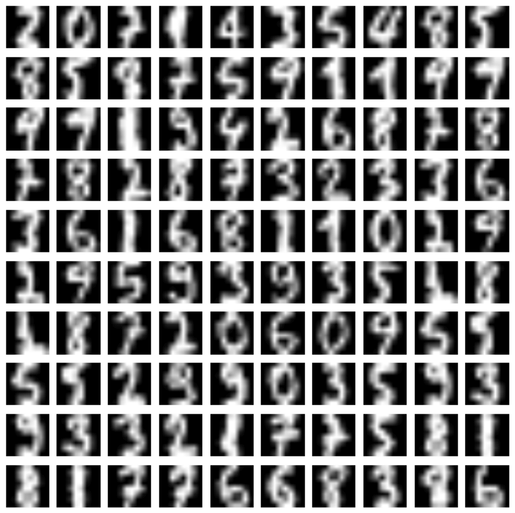
A figure with a few random MNIST handwritten digits is shown as follows:一些MNIST手写数字图像显示如下:
 A plot for the example of MNIST digits is shown next. The left graph represents the variance ratio while the right one is the cumulative variance. It can be immediately seen how the first components are normally the most important ones in terms of information, while the following ones provide details that a classifier could also discard:MNIST数字样本作图如下。左侧代表方差比而右侧代表累积方差。可以立即看到,在信息方面,第一个成分通常是最重要的成分,而下面的成分提供了分类器也可以丢弃的细节:
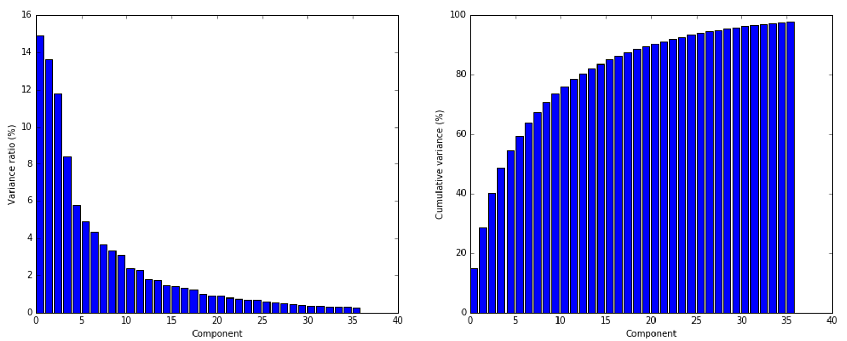 As expected, the contribution to the total variance decreases dramatically starting from the fifth component, so it's possible to reduce the original dimensionality without an unacceptable loss of information, which could drive an algorithm to learn wrong classes.正如预期的那样,从第5个成分开始,对总方差的贡献会急剧减少,因此可以降低原始维数,又不至于造成难以接受的信息损失,难以接受的信息损失将导致算法学习错误的类。
The result is shown in the following figure:(经PCA转换)结果显示如下:
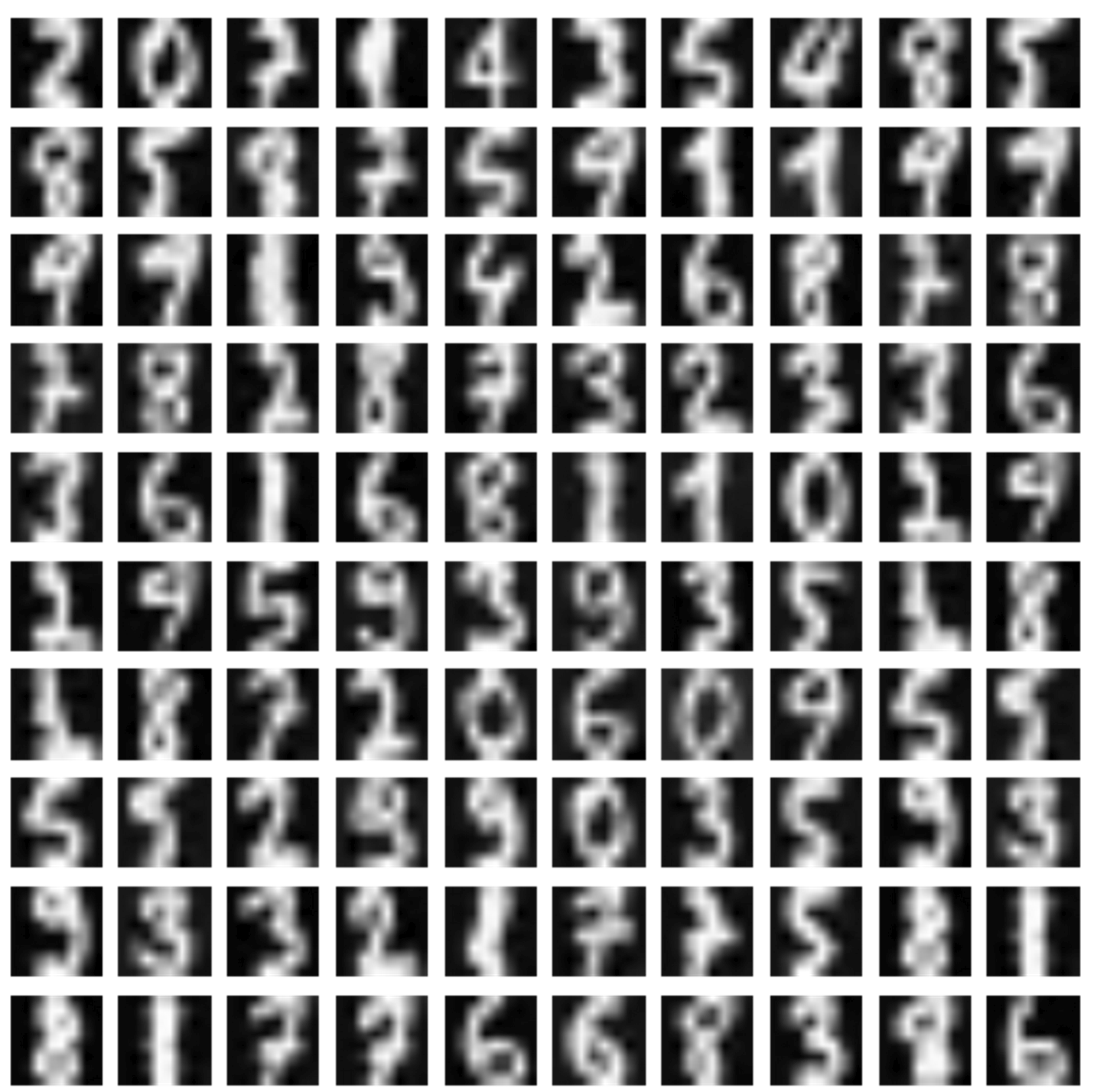 This process can also partially denoise the original images by removing residual variance, which is often associated with noise or unwanted contributions (almost every calligraphy distorts some of the structural elements which are used for recognition).这个过程(指PCA)也可部分降噪 这个过程还可以通过去除残差来部分地降噪原始图像,残差通常与噪声或不必要的贡献相关联(几乎每一幅书法作品都会扭曲用于识别的某些结构元素)。
【 请阅读pca原理
经PCA转换后的矩阵:
- 列向量线性无关;
- 维度减少。 】
3.7.1 Non-negative matrix factorization非负矩阵分解(NNMF)
When the dataset is made up of non-negative elements, it's possible to use non-negative matrix factorization (NNMF) instead of standard PCA. The algorithm optimizes a loss function (alternatively on W and H) based on the Frobenius norm:当数据集由非负元素组成,可以由标准PCA改用非负矩阵分解(NNMF)。算法优化基于Frobenius范数的损失函数(在W和H上交替进行):

$$L = \frac{1}{2} {||\mathbf{X-WH}||}_{Frob}^2 \ where \ {||\mathbf{A}||}_{Frob}^2 = \sqrt{\sum_{i}\sum_{j} {|a_{ij}|^2}}$$
算法什么意思呢?用WH来代表原始特征矩阵。W和H均是非负矩阵,且需要W的列数小于X的列数。随意初始比如W、H为某非负矩阵,交替优化以使X-WH的Frobenius范数小到令我们满意。
If dim(X) = $n \times m$, then dim(W) = $n \times p$ and dim(H) = $p \times m$ with p equal to the number of requested components (the n_components parameter), which is normally smaller than the original dimensions n and m.如果dim(X) = $n \times m$, 那么dim(W) = $n \times p$, dim(H) = $p \times m$, p等于所请求的成分数(n_components参数),通常小于原尺寸n和m。
The final reconstruction is purely additive and it has been shown that it's particularly efficient for images or text where there are normally no non-negative elements.最后的重构是纯加法的,它已经被证明对于通常没有非负元素的图像或文本特别有效。
【 请阅读nmf或者叫nnmf原理
经稀疏PCA转换后的矩阵:
- 列向量线性无关;
- 维度减少;
- 分解出的两个矩阵只要有一个所有值非负。 】
3.7.2 Sparse PCA稀疏主成分分析
SparsePCAallows exploiting the natural sparsity of data while extracting principal components.If you think about the handwritten digits or other images that must be classified, their initial dimensionality can be quite high (a 10x10 image has 100 features). However, applying a standard PCA selects only the average most important features, assuming that every sample can be rebuilt using the same components. Simplifying, this is equivalent to:SparsePCA允许利用自然稀疏的数据,同时提取主成分。如果你考虑手写数字或其他必须分类的图像,它们的初始维度可能相当高(10x10的图像有100个特征)。然而,应用标准PCA只选择最重要的平均特征,假设每个样本都可以使用相同的成分重新构建。化简,这等于:

$$y_R = C_1 \cdot y_{R1} +C_2 \cdot y_{R2}+ \dots + C_g \cdot y_{Rg}$$
注意上式左边是原始数据中一个元素,右式是g个主成分对这个元素的模拟
On the other hand, we can always use a limited number of components, but without the limitation given by a dense projection matrix. This can be achieved by using sparse matrices (or vectors), where the number of non-zero elements is quite low. In this way, each element can be rebuilt using its specific components (in most cases, they will be always the most important), which can include elements normally discarded by a dense PCA. The previous expression now becomes:另一方面,我们总是可以使用有限数量的成分,但不用限制为稠密投影矩阵。这可以通过使用稀疏矩阵(或向量)来实现,其中非零元素的数量相当少。通过这种方式,每个元素都可以使用其特定的成分进行重建(在大多数情况下,这些成分总是最重要的),成分可以包含通常被稠密的PCA丢弃的元素。上式现在变为:

$$y_R = C_1 \cdot y_{R1} +C_2 \cdot y_{R2}+ \dots + C_g \cdot y_{Rg} + (0 \cdot y_{Rg+1} +0 \cdot y_{Rg+2}+ \dots + 0 \cdot y_{Rm})$$
注意上式左边是原始数据中一个元素,由式是m个成分对这个元素的模拟。m就是原始数据的特征数。看这里会以为稀疏pca不能降维,其实稀疏pca也能降维。
Here the non-null components have been put into the first block (they don't have the same order as the previous expression), while all the other zero terms have been separated. In terms of linear algebra, the vectorial space now has the original dimensions. However, using the power of sparse matrices (provided by scipy.sparse), scikit-learn can solve this problem much more efficiently than a classical PCA.在这里,非空组件被放在第一个块中(它们的顺序与前一个表达式不一样),而所有其他的零项被分开。在线性代数中,矢量空间现在有了原始的维数。然而,使用稀疏矩阵(由scipy.sparse提供)的能量,scikit-learn可以比传统的PCA更有效地解决这个问题。
稀疏PCA也能降维并稀疏转换后的矩阵,之后可以靠scipy.sparse实现良好的运算速度。
【 请阅读稀疏pca原理
经稀疏PCA转换后的矩阵:
- 列向量线性无关;
- 维度减少;
- 稀疏。 】
datetime: 2018/11/19 0:07
3.7.3 Kernel PCA核主成分分析
KernelPCA performs a PCA with non-linearly separable data sets. Just to understand the logic of this approach (the mathematical formulation isn't very simple), it's useful to consider a projection of each sample into a particular space where the dataset becomes linearly separable. The components of this space correspond to the first, second, ... principal components and a kernel PCA algorithm, therefore, computes the projection of our samples onto each of them. KernelPCA使用非线性可分数据集执行PCA。为了理解这种方法的逻辑(数学公式不是很简单),考虑将每个样本投影到使数据集线性可分的特定空间是很有用的。这个空间的成分对应于第一,第二,…主成分和一个核PCA算法,然后,计算我们的样本在空间每一个成分上的投影。
线性可分就是说可以用一个线性函数把两类样本分开,比如二维空间中的直线、三维空间中的平面以及高维空间中的线型函数。
The graphical representation is shown in the following picture. In this case, a classic PCA approach isn't able to capture the non-linear dependency of existing components (the reader can verify that the projection is equivalent to the original dataset). However, looking at the samples and using polar coordinates (therefore, a space where it's possible to project all the points), it's easy to separate the two sets, only considering the radius:图示如下图所示。在这种情况下,经典的PCA方法不能捕获现有组件的非线性依赖关系(读者可以验证投影是否等于原始数据集。确实,经典PCA的投影下投影等价于源数据,仍然是大环包圆心)。然而,观察样本并使用极坐标(即一个可以投射所有点的空间),只考虑半径,很容易将两个集合分开:
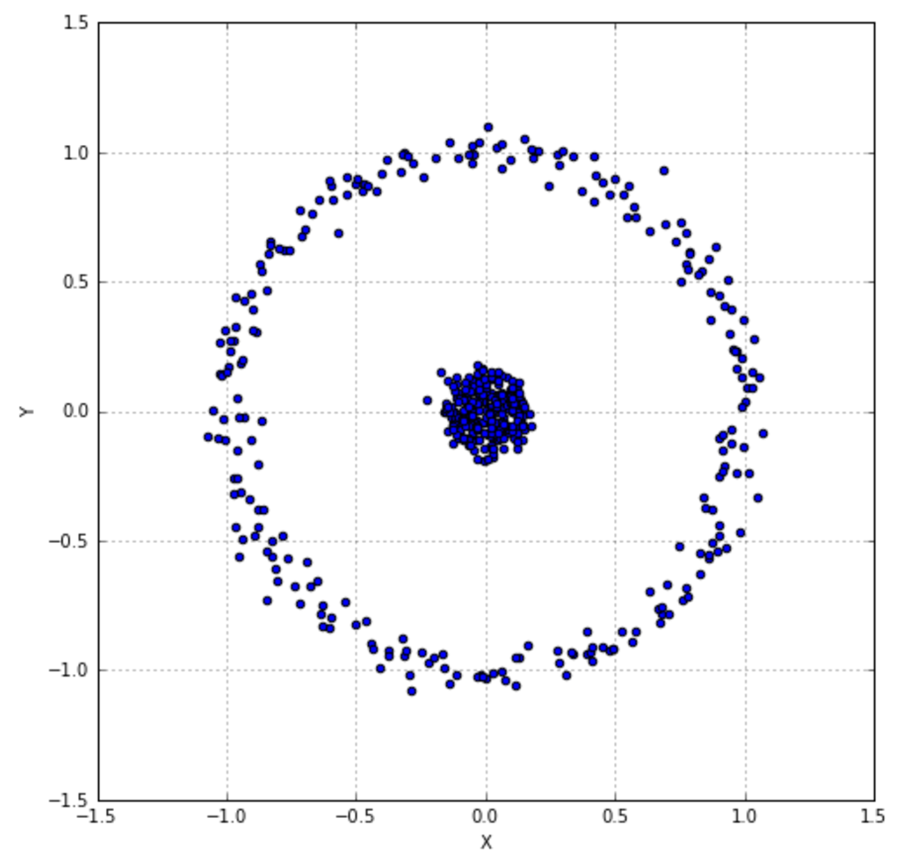 Plotting it, we get:画图后如下:
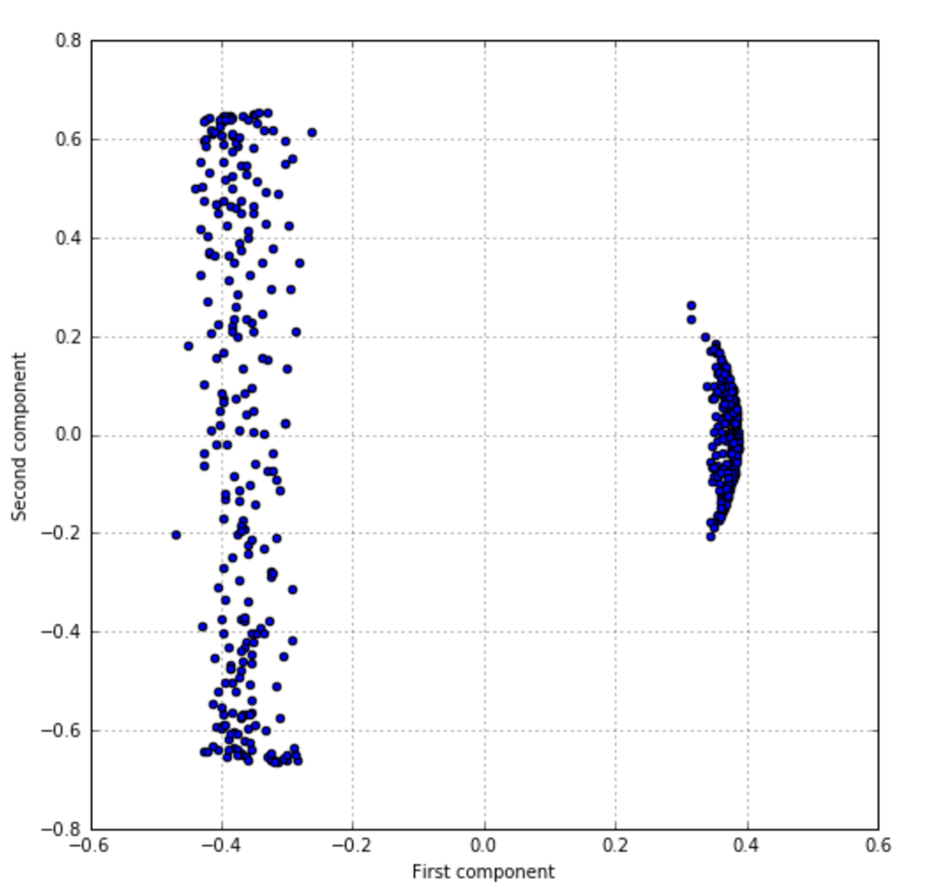 The plot shows a separation just like expected, and it's also possible to see that the points belonging to the central blob have a curve distribution because they are more sensitive to the distance from the center.上图显示了与预期一样的分离,也可以看到属于中心团的点具有曲线分布,因为它们对到圆心的距离更敏感。
Kernel PCA is a powerful instrument when we think of our dataset as made up of elements that can be a function of components (in particular, radial-basis or polynomials) but we aren't able to determine a linear relationship among them.当我们怀疑数据集符合某个成分函数(特别是径向基或多项式)且无法找到数据元素的线性关系,那么核PCA将是有力工具。
【
采用核方法,相当于从数据矩阵的特征列的集合中选取k列特征(k可以为1到m的任意整数),这是一个新的矩阵,对这个矩阵的两行计算相似度,这个相似度是一个新的特征列,那么相似度形成的特征列将最多有$2^m$列。相似度特征列可以考虑加进原数据列,也可以替换原数据列。经核方法的数据列将最多有$m+2^m$列,接下进行正常的PCA,这就是核PCA的原理。
关于核方法可阅读我的摘抄博文核方法kernel_method。
】
【 我对pca的总结 】
datetime: 2018/11/20 21:37
3.8 Atom extraction and dictionary learning原子提取和字典学习
Dictionary learning is a technique which allows rebuilding a sample starting from a sparse dictionary of atoms (similar to principal components)。 which can be summarized as a double optimization problem where:字典学习是一种技术,它允许从稀疏的原子字典(类似于主成分)重新构建样本。可以概括为一个双重优化问题:

$$\mathbf{X}=\{\vec{x}_1,\vec{x}_2,\ldots,\vec{x}_n\} \ where \ \vec{x}_i \in \mathbb{R}^m$$
Is an input dataset and the target is to find both a dictionary D and a set of weights for each sample:(上式)是个输入数据集且目标是查找字典D和对应每个样本的一组权重:

$$\mathbf{D} \in \mathbb{R}^{n \times k} \ and \ \mathbf{A}=\{\vec{\alpha}_1,\vec{\alpha}_2, \ldots, \vec{\alpha}_m\} \ where \ \vec{\alpha}_i \in \mathbb{R}^{k}$$
其实字典学习就是稀疏PCA,将$\mathbf{X}_{n \times m}$分解为$\mathbf{D}_{n \times k}\mathbf{A}_{k \times m}$。作者这里公式有点小错误,我改过来了。
After the training process, an input vector can be computed as:经过训练过程,输入向量可以计算为:

$$\vec{X}_i=\mathbf{D}\vec{\alpha}_i$$
The optimization problem (which involves both D and alpha vectors) can be expressed as the minimization of the following loss function:优化问题(涉及D和alpha向量)可以表示为以下损失函数的最小化:

$$L(\mathbf{D},\mathbf{A})=\frac{1}{2}\sum_{i}{\|\vec{X}_i-\mathbf{D}\vec{\alpha}_i\|_2^2+c\|\vec{\alpha}_i\|_1}$$
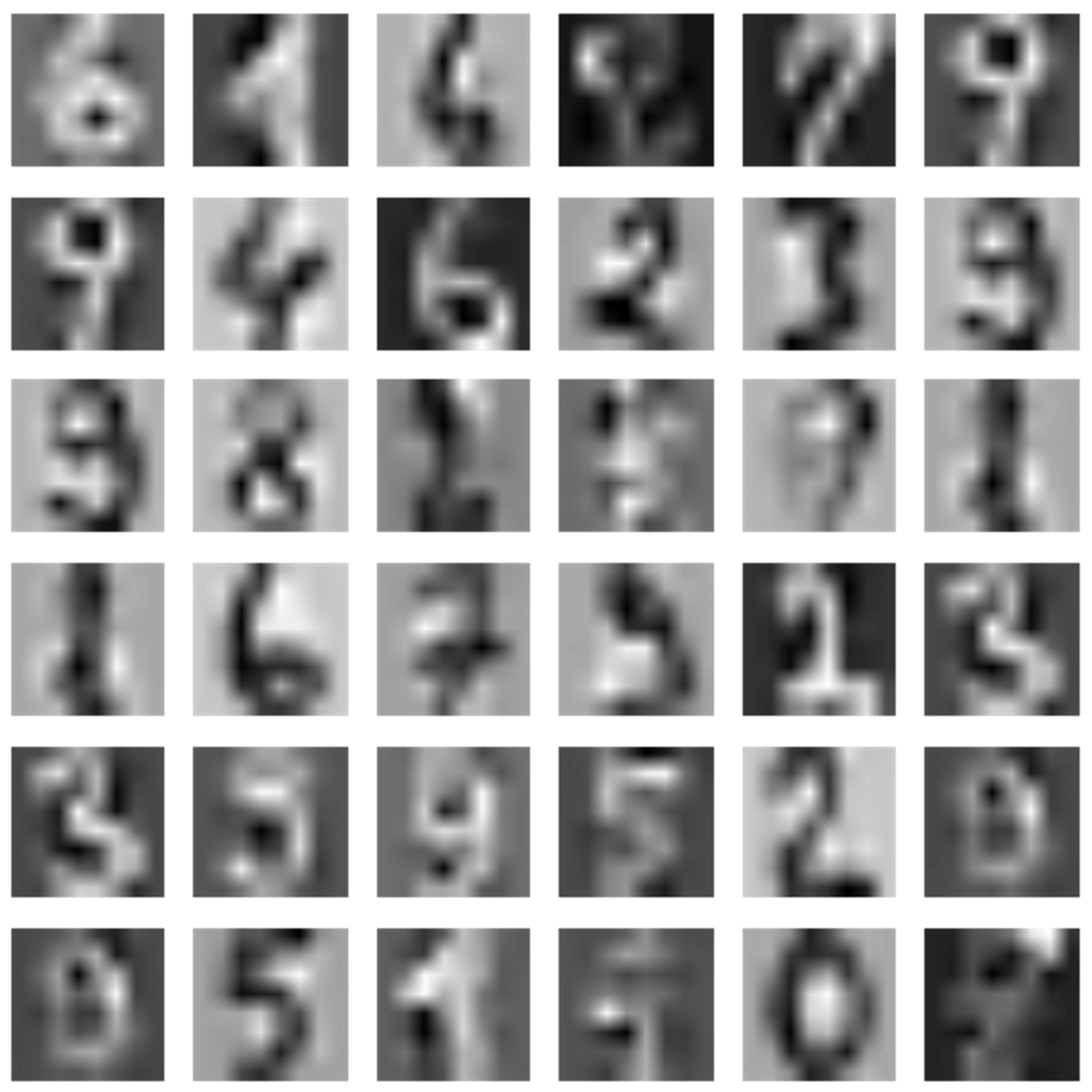
Here the parameter c controls the level of sparsity (which is proportional to the strength of L1 normalization). This problem can be solved by alternating the least square variable until a stable point is reached.在这里,参数c控制稀疏程度(稀疏程度与L1归一化强度成正比)。这个问题可以通过变换最小二乘变量来解决,直到到达一个稳定点。
A plot of each atom (component) is shown in the following figure:每个原子(成分)的图如下图所示:
3.9 References参考文献
3.10 Summary总结
4 Linear Regression线性回归
4.1 Linear models线性模型
Consider a dataset of real-values vectors:考虑一个由实数向量组成的数据集:

$$\mathbf{X}=\{\vec{x}_1,\vec{x}_2,\ldots,\vec{x}_n\} \ where \ \vec{x}_i \in \mathbb{R}^m$$
Each input vector is associated with a real value yi:每个输入向量都与一个实值yi相关联:

$$y=\{y_1,y_2,\ldots,y_n\} where \ y_n \in \mathbb{R}$$
A linear model is based on the assumption that it's possible to approximate the output values through a regression process based on the rule:线性模型是基于这样的假设,即可以通过基于规则的回归过程逼近输出值:

$$\hat{y}=\alpha_0 + \sum_{i=1}^{m}{\alpha_ix_i} \ where \ A=\{\alpha_0,\alpha_0,\ldots,\alpha_m\}$$
In other words, the strong assumption is that our dataset and all other unknown points lie on a hyperplane and the maximum error is proportional to both the training quality and the adaptability of the original dataset. One of the most common problems arises when the dataset is clearly non-linear and other models have to be considered (such as neural networks or kernel support vector machines).换句话说,强假设为:我们的数据集和所有其他未知点都位于超平面上,最大误差与训练质量和原始数据集的适应性成正比。当数据集明显是非线性的并且必须考虑其他模型(如神经网络或核支持向量机)时,最常见的问题之一就出现了。
4.2 A bidimensional example一个二维的例子
In the following figure, there's a plot with a candidate regression function:在下面的图中,有一个带有候选回归函数的图:
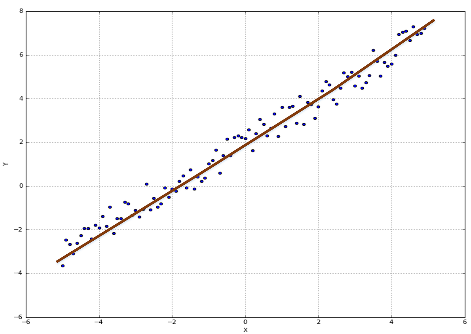 As we're working on a plane, the regressor we're looking for is a function of only two parameters:既然是平面,那么我们要找的回归函数只有两个参数:

$$\hat{y}=\alpha + \beta x$$
In order to fit our model, we must find the best parameters and to do that we choose an ordinary least squares approach. The loss function to minimize is:为了适合我们的模型,我们必须找到最佳的参数,为此我们选择了一个普通的最小二乘法(普通最小二乘法(又称最小平方法)是一种数学优化技术。它通过最小化误差的平方和寻找数据的最佳函数匹配。其实等效于机器学习里面采用均方差损失函数)。要最小化的损失函数是:

$$L=\frac{1}{2n}{\sum_{i=1}^{n}{\|\hat{y}_i-y_i\|_2^2}} \ which \ becomes \ L=\frac{1}{2n}{\sum_{i=1}^{n}{(\alpha+\beta x_i-y_i)^2}}$$
除n
With an analytic approach, in order to find the global minimum, we must impose:用分析的方法,为了找到全局最小值,我们必须利用:
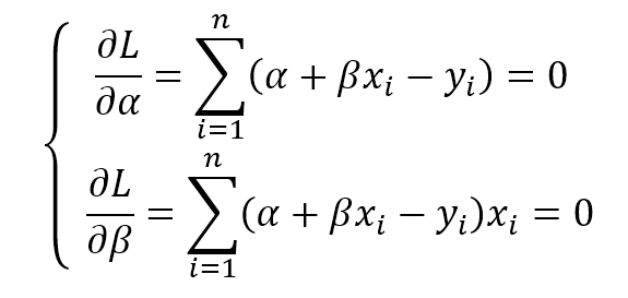
$$\left\{ \begin{aligned} \frac{\partial{L}}{\partial{\alpha}} & =\sum_{i=1}^{n}{(\alpha+\beta x_i - y_i)}=0 \\ \frac{\partial{L}}{\partial{\beta}} & =\sum_{i=1}^{n}{(\alpha+\beta x_i - y_i)x_i}=0 \end{aligned} \right.$$
4.3 Linear regression with scikit-learn and higher dimensionality利用scikit-learn且更高维度的线性回归
It (Boston dataset) has 506 samples with 13 input features and one output. In the following figure, there' a collection of the plots of the first 12 features:它(波士顿数据集)有506个示例,13个输入特性和一个输出。在下面的图中,我们收集了前12个特性的图:
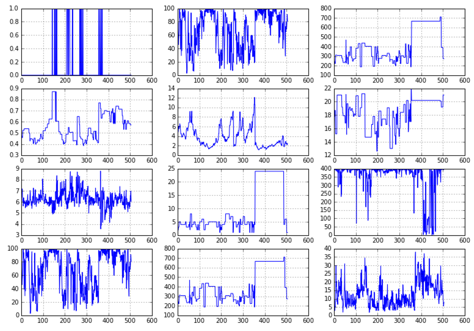 When the original data set isn't large enough, splitting it into training and test sets may reduce the number of samples that can be used for fitting the model. k-fold cross-validation can help in solving this problem with a different strategy. The whole dataset is split into k folds using always k-1 folds for training and the remaining one to validate the model. K iterations will be performed, using always a different validation fold. In the following figure, there's an example with 3 folds/iterations:当原始数据集不够大时,将其分为训练集和测试集可能会减少用于拟合模型的样本数量。k-fold交叉验证可以用(是指简单交叉验证将损失一部分拟合数据,而k-fold不会,这点是不同的)不同的策略帮助解决这个问题。整个数据集被分割成k个部分,使用总是k-1个部分进行训练,剩下部分用于验证模型。将执行K次迭代,始终使用不同的验证部分。下图是一个3部分/迭代的例子:
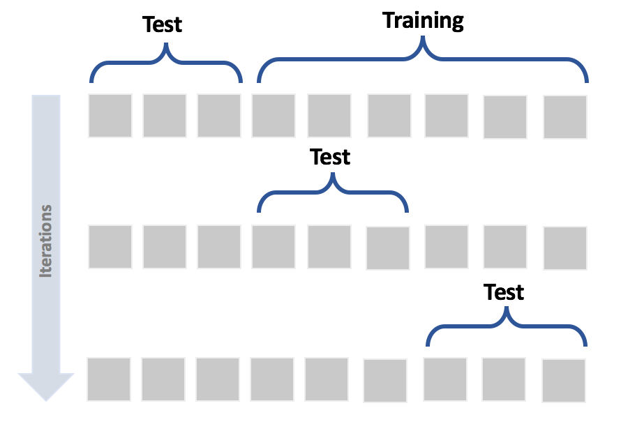 In this way, the final score can be determined as average of all values and all samples are selected for training k-1 times.这样,最终的分数可以定为所有值的平均值,并且所有的样本被选中进行k-1次训练。
k-fold适用于样本较少时候,不是只适用于线性回归!
Another very important metric used in regressions is called the coefficient of determination or R2. It measures the amount of variance on the prediction which is explained by the dataset. We define residuals, the following quantity:回归分析中使用的另一个非常重要的指标叫做可决系数或R2。它测量了由数据集解释的预测的方差量。我们定义残差,如下量:

$$\forall i \in (0,n) \ r_i=x_i-\hat{x}_i$$
In other words, it is the difference between the sample and the prediction. So the R2 is defined as follows:也就是样本和预测之间的差异。所以R2定义如下:

$$R^2=1-\frac{\sum_{i}{r_i^2}}{\sum_{i}{(x_i-E[\mathbf{X}])}}$$
上面两个表达式中用了x,其实用y更适合我们理解,y的实际值和预测值。
For our purposes, R2 values close to 1 mean an almost perfect regression, while values close to 0 (or negative) imply a bad model. 就我们的目的而言,R2接近1的值意味着近乎完美的回归,而接近0(或负)的值意味着坏的模型。
注意loss function和metric的区别:其实数学上是一个东西,只是loss function将用于更新模型和评估效果,而metric只用于评估效果。当然,更精确说法,在很多package里面是一回事,但catboost、lightgbm、xgboost里面,由于为了计算效率,其优化项用泰勒公式来近似,此时loss函数返回的其实是同时返回优化项的一阶导数和二阶导数。
4.3.1 Regressor analytic expression回归量解析表达式
其实是在讲怎么获得训练后的参数,这样也就得到了解析表达式。用scikit-learn很简单,略。
不过,本节提到,普通最小二乘法模型,如果效果不好,无外乎三种原因: 1.数据不适合线性模型。 2.数据存在域外值。 3.数据特征列之间的共线性。这将导致数据对噪声很敏感,造成一些参数爆炸。解决办法就是规范这些参数,如4.4节的手段。
4.4 Ridge, Lasso, and ElasticNet岭回归、套索回归、松紧带回归
Ridge regression imposes an additional shrinkage penalty to the ordinary least squares loss function to limit its squared L2 norm:岭回归对普通最小二乘损失函数施加额外的收缩惩罚以限制其平方L2范数:
alpha是惩罚力度,限制参数大小的增长

$$L(\vec{w})=\frac{1}{2n}\|\mathbf{X}\vec{w}-\vec{y}\|_2^2+\alpha\|\vec{w}\|_2^2$$
In the following figure, there's a representation of what happens when a Ridge penalty is applied:下图示意应用岭惩罚项时会发生什么:
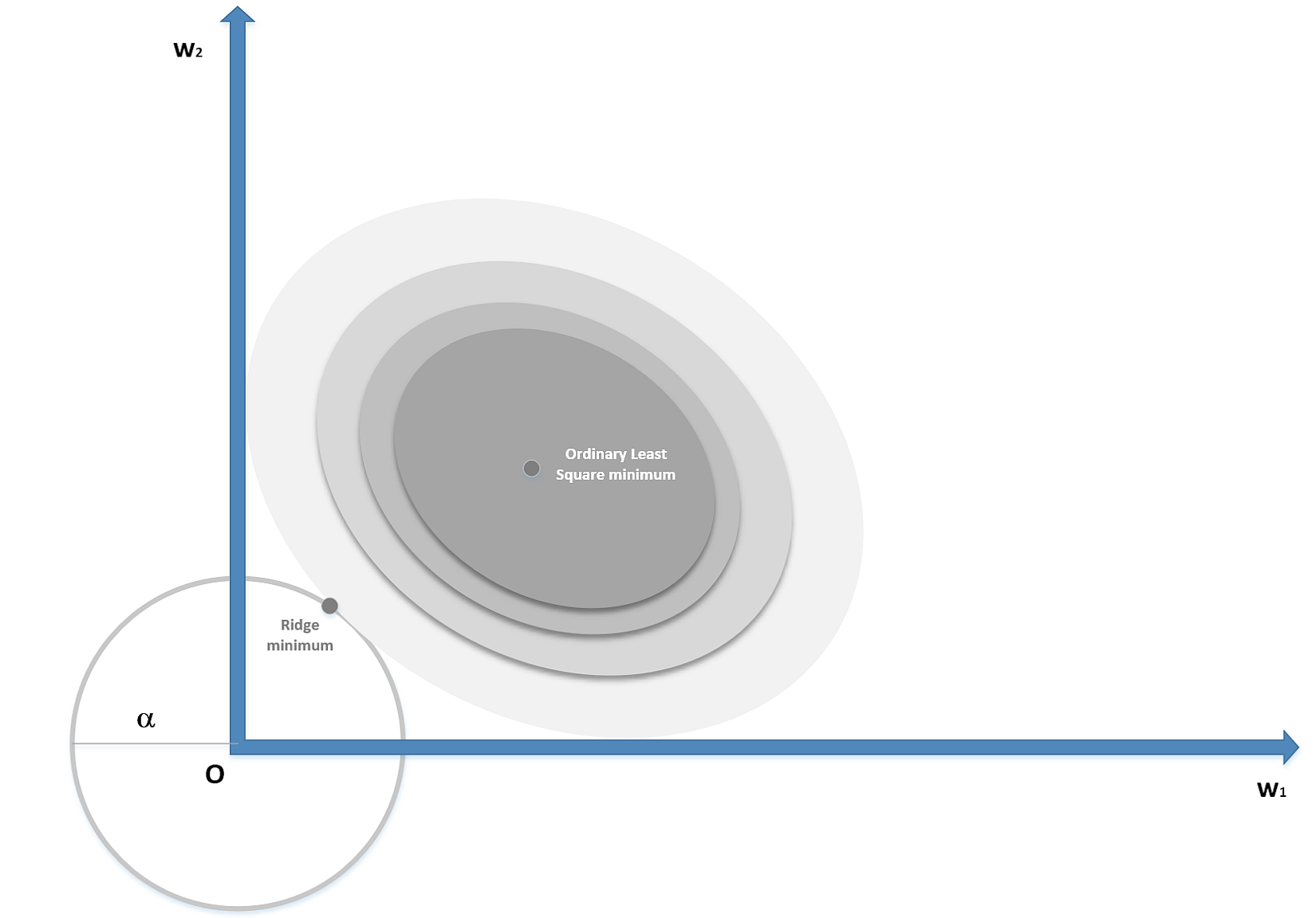 The gray surface represents the loss function (here, for simplicity, we're working with only two weights), while the circle center O is the boundary imposed by the Ridge condition. The minimum will have smaller w values and potential explosions are avoided.灰色的表面表示损失函数(这里,为了简单起见,我们只使用了两个权值),而圆O是山脊条件施加的边界。最小值的w(这时也就是
$w_1$和$w_2$)值更小,避免了潜在的爆炸。
上图:如果没有参数惩罚项,那就是普通最小二乘法回归,能达到的最低训练损失对应的参数在一个等高线上,根据噪声等,可能在参数较小的地方也可能在参数很大的地方;如果加入岭惩罚项,那就是岭回归,岭回归的训练损失相对普通最小二乘法回归要大一点,好处就是参数被惩罚项限制了,参数项随机减少而且参数项值相对更小。惩罚项前参数越大,惩罚力度越大,参数随机性越小参数项值越小。
刚发现,居然可以通过网格搜索找到最优惩罚项前的参数,这个参数本来是高参。
A Lasso regressor imposes a penalty on the L1 norm of w to determine a potentially higher number of null coefficients:套索回归对w施加L1范数惩罚,以使参数出现更多零系数:
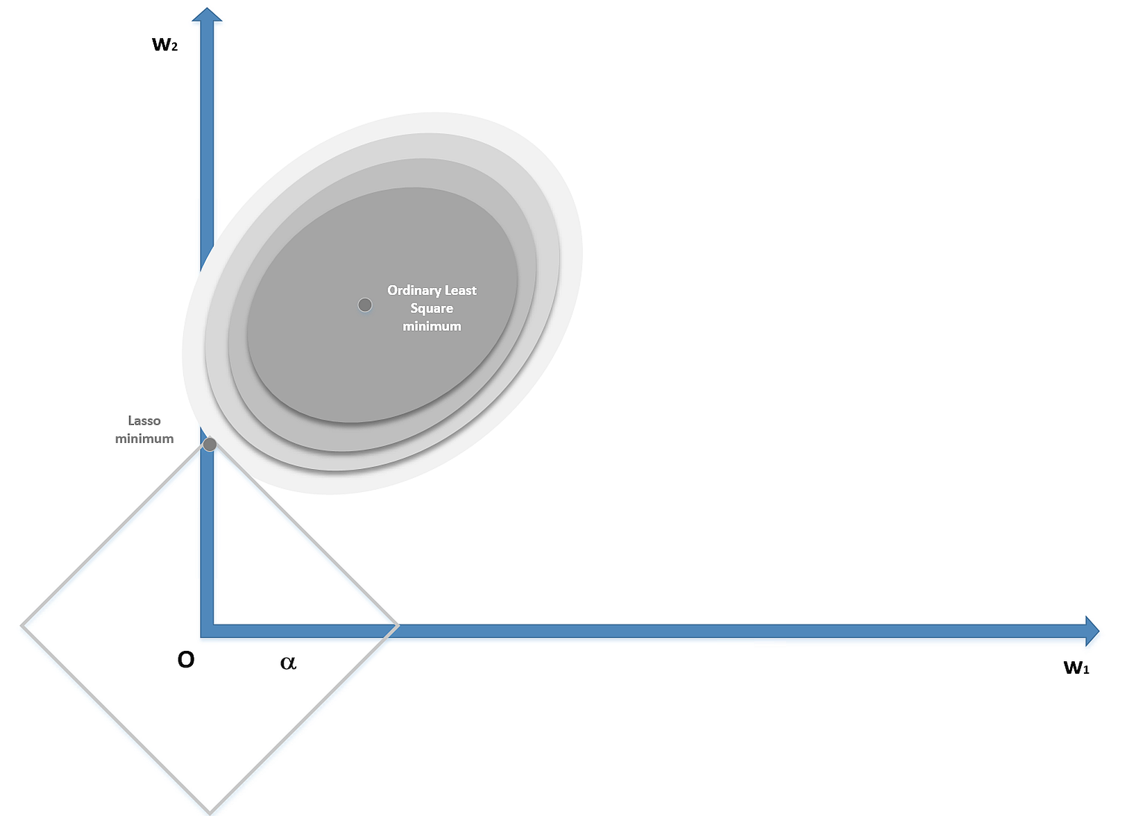 The sparsity is a consequence of the penalty term (the mathematical proof is non-trivial and will be omitted).稀疏性是惩罚项的结果(数学证明是非平凡的,将被省略)。

$$L(\vec{w})=\frac{1}{2n}\|\mathbf{X}\vec{w}-\vec{y}\|_2^2+\alpha\|\vec{w}\|_2^2$$
In this case, there are vertices where a component is non-null while all the other weights are zero. The probability of an intersection with a vertex is proportional to the dimensionality of w and, therefore, it's normal to discover a rather sparse model after training a Lasso regressor.在这种情况下,有一些顶点,其中一个组件是非空的,而所有其他权重都为零。与顶点相交的概率与w的维数成正比,因此,在训练套索回归后发现一个相当稀疏的模型是很正常的。
刚发现,居然可以通过网格搜索找到最优惩罚项前的参数,这个参数本来是高参。
The last alternative is ElasticNet, which combines both Lasso and Ridge into a single model with two penalty factors: one proportional to L1 norm and the other to L2 norm. In this way, the resulting model will be sparse like a pure Lasso, but with the same regularization ability as provided by Ridge. The resulting loss function is:最后是松紧带回归,即在模型中同时包岭惩罚项和套索惩罚项:一个与L1成正比,另一个与L2成正比。这样,生成模型将如纯套索回归一样稀疏,但但具有岭回归一般的正则化能力。松紧带回归的损失函数是:

$$L(\vec{w})=\frac{1}{2n}\|\mathbf{X}\vec{w}-\vec{y}\|_2^2+\alpha\beta\|\vec{w}\|_1+\frac{\alpha(1-\beta)}{2}{\|\vec{w}\|_2^2}$$
刚发现,居然可以通过网格搜索找到最优惩罚项前的参数,这个参数本来是高参。
4.5 Robust regression with random sample consensus采用随机样本一致的鲁棒性回归
A common problem with linear regressions is caused by the presence of outliers. An ordinary least square approach will take them into account and the result (in terms of coefficients) will be therefore biased. In the following figure, there's an example of such a behavior:线性回归的一个常见问题是由域外值的存在引起的。一个普通的最小二乘方法会计入域外值,因此结果(在系数方面)会有偏差。在下面的图中,有一个这样的行为的例子:
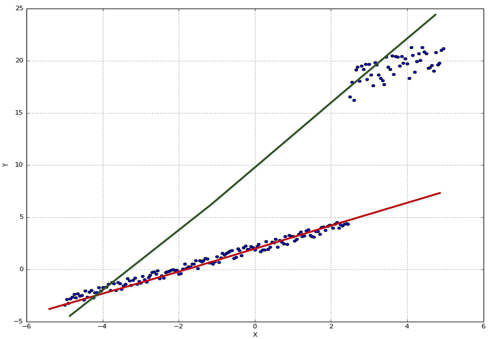 The less sloped line represents an acceptable regression which discards the outliers, while the other one is influenced by them. An interesting approach to avoid this problem is offered by random sample consensus (RANSAC), which works with every regressor by subsequent iterations, after splitting the dataset into inliers and outliers. The model is trained only with valid samples (evaluated internally or through the callable
 is_data_valid()) and all samples are re-evaluated to verify if they're still inliers or they have become outliers. The process ends after a fixed number of iterations or when the desired score is achieved.不那么倾斜的直线代表一个可接受的回归,它丢弃了域外值,而另一个受到域外值的影响。随机样本一致(RANSAC)提供了一种避免这个问题的有趣方法,它在将数据集分成非离群值和离群值之后,通过后续迭代对每个回归子进行处理。模型只使用有效的样本(内部评估或通过调用is_data_valid())进行训练,所有的样本都要重新评估,以验证它们是否仍然是正常值,或者它们已经成为域外值。这个过程在固定的迭代次数或达到期望的分数之后结束。
查阅sklearn文档,鲁棒性回归将数据点分成非离群值和离群值,将务求使离群值更少。其需要接受一个基础回归器作为参数。而且,当特征过多时,效果不佳。
4.6 Polynomial regression多项式回归
Polynomial regression is a technique based on a trick that allows using linear models even when the dataset has strong non-linearities. The idea is to add some extra variables computed from the existing ones and using (in this case) only polynomial combinations:多项式回归是一种基于技巧的技术,使得即使数据集具有很强的非线性,也可以使用线性模型。其思想是添加一些从现有变量中计算出来的额外变量,并且额外变量经多项式组合而来。

$$\hat{y}=\alpha_0+\sum_{i=i}^{m}{\alpha_ix_i}+\sum_{j=m+1}^{k}{\alpha_jf_{Pj}(x_1,x_2,\ldots,x_m)} \\ where \ f_{Pj} \text{ is a polynormial function}$$
For example, with two variables, it's possible to extend to a second-degree problem by transforming the initial vector (whose dimension is equal to m) into another one with higher dimensionality (whose dimension is k > m):例如,对于两个变量,可以通过将初始向量(其维数为m)转换为另一个维度更高的向量(其维数为k > m)来扩展到二阶问题。

$$\vec{x}=[x_1,x_2] \Rightarrow \\ \vec{x}_t=[x_1,x_2,x_1^2,x_2^2,x_1x_2]$$
In this case, the model remains externally linear, but it can capture internal non-linearities. To show how scikit-learn implements this technique, let's consider the dataset shown in the following figure:在这种情况下,模型仍然是外部线性的,但它可以捕获内部非线性。为了展示scikit-learn如何实现这种技术,让我们考虑如下图所示的数据集:
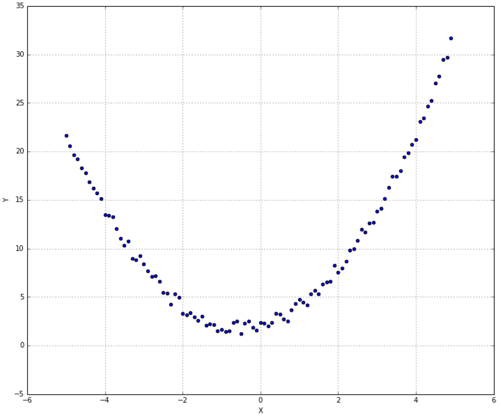 The score is quite higher and the only price we have paid is an increase in terms of features. In general, this is feasible; however, if the number grows over an accepted threshold, it's useful to try a dimensionality reduction or, as an extreme solution, to move to a non-linear model (such as SVM-Kernel).(多项式回归)得分很高,只是会增加特征项。一般来说,这是可行的;但是,如果数字增长超过了一个可接受的阈值,那么尝试降维或者作为一种极端的解决方案转向非线性模型(比如SVM-Kernel)是很有用的。
4.7 Isotonic regression保序回归
There are situations when we need to find a regressor for a dataset of non-decreasing points which can present low-level oscillations (such as noise). A linear regression can easily achieve a very high score (considering that the slope is about constant), but it works like a denoiser, producing a line that can't capture the internal dynamics we'd like to model. For these situations, scikit-learn offers the class IsotonicRegression, which produces a piecewise interpolating function minimizing the functional:在某些情况下,我们需要为非递减点数据集找到一个回归方程,这些数据集可能会出现低水平的振荡(如噪声)。线性回归可以很容易地获得很高的分数(考虑到斜率是常数),但它的工作方式就像去噪器一样,产生的直线无法捕捉我们希望捕捉到的内部动态。对于这些情况,scikit-learn提供了IsotonicRegression,它产生一个分段插值函数,使泛函数最小化:

$$L=\sum_{i}{w_i(y_i-\hat{y}_i)^2} \ where \ y_0 \le y_1 \le \dots \le y_n$$
【
The isotonic regression optimization problem is defined by:保序回归问题定义如下:
$$min \sum_{i=1}^{n} w_i (y_i - \hat{y}_i)^2 \\
subject \ to \ y_i \le y_j \ whenever \ x_i \le x_j$$
where:
$y_i$are inputs (real numbers)$y_i$是输入(实数)$\hat{y}_i$are fitted$\hat{y}_i$是训练后的$x$specifies the order. If$x$is non-decreasing then$\hat{y}$is non-decreasing.$x$指定顺序。如果$x$不递减,那么$\hat{y}$不递减。按sklearn目前源代码暂时x必须只含1个特征(1d array),保序回归是按照x指定顺序的,若含有多个特征列,不好确定顺序。$w_i$are optional strictly positive weights (default to 1.0)$w_i$是可选的严格正值(默认为1.0)
根据sklearn文档,保序回归是非参数学习($w_i$是高参)。学习的是预测值的大小,预测值需要保序(也就是单调,注意,不一定非递减。)
】
Following is a plot of the dataset. As everyone can see, it can be easily modeled by a linear regressor, but without a high non-linear function, it is very difficult to capture the slight (and local) modifications in the slope:下面是数据集的一个图。正如大家所见,它可以很容易地用线性回归函数来建模,但是如果没有高非线性函数,就很难捕捉到斜率的细微(和局部)变化,
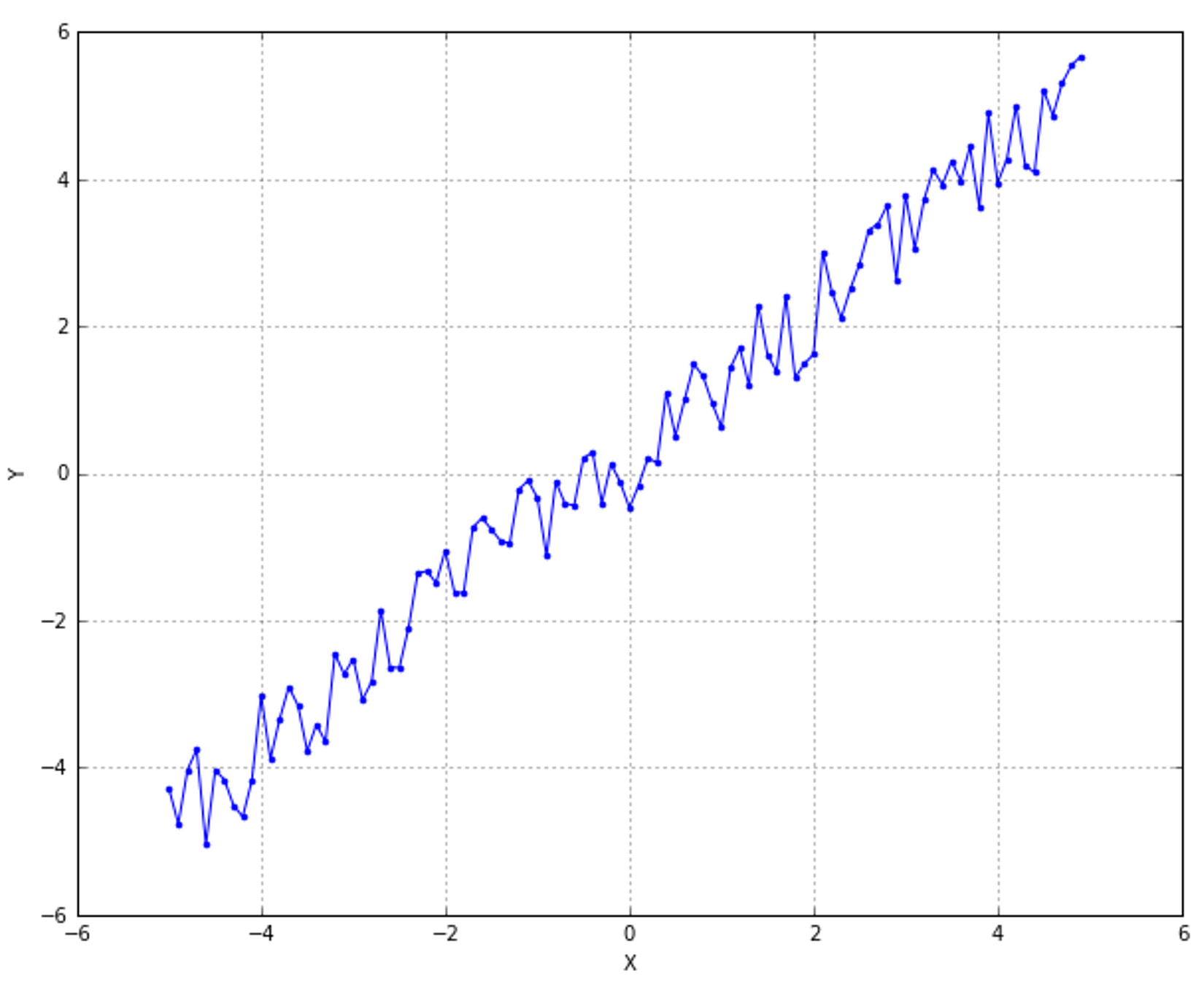 The class
 IsotonicRegression needs to know ymin and ymax (which correspond to the variables y0 and yn in the loss function). In this case, we impose -6 and 10:IsotonicRegression需要知道ymin和ymax(对应于损失函数中的变量y0和yn)。在这种情况下,我们设置-6和10:
A plot of this function (the green line), together with the original data set, is shown in the following figure:这个函数(绿线)和原始数据集的示意图如下图所示:
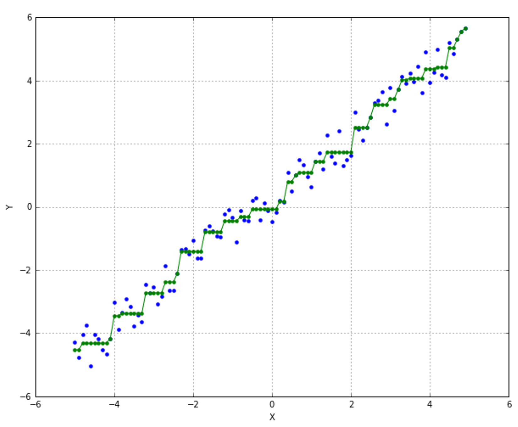
datetime 2018/11/20 17:51
4.8 References参考文献
4.9 Summary总结
5 Logistic Regression逻辑回归
5.1 Linear classification线性分类
Let's consider a generic linear classification problem with two classes. In the following figure, there's an example:让我们考虑一个有两个类的一般线性分类问题。在下面的图中,有一个例子:
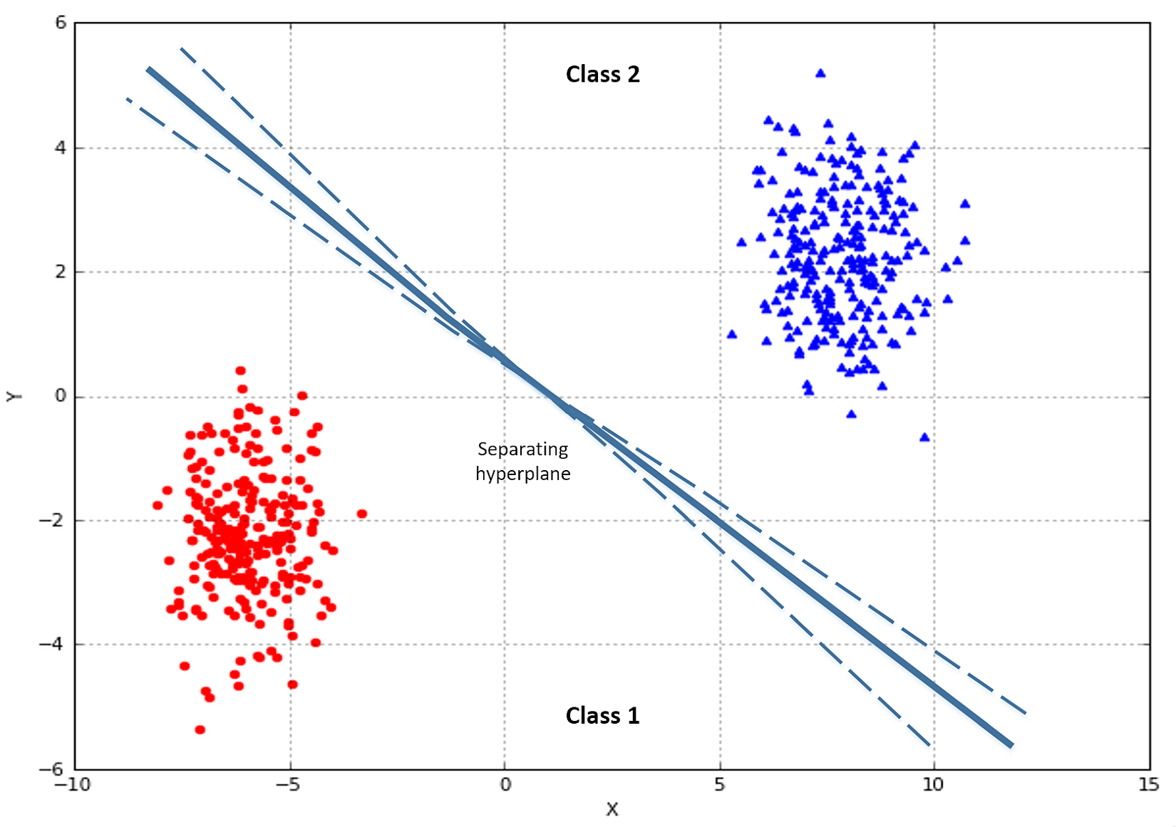 Our goal is to find an optimal hyperplane, which separates the two classes. In multi-class problems, the strategy one-vs-all is normally adopted, so the discussion can be focused only on binary classifications. Suppose we have the following dataset:我们的目标是找到一个最优超平面,将这两个类分开。在多类问题中,通常采用one-vs-all策略,因此讨论可以只集中在二元分类上。假设我们有如下数据集:

$$\mathbf{X}=\{\vec{x}_1,\vec{x}_2,\ldots,\vec{x}_n\} \ where \ \vec{x}_i \in \mathbb{R}^m$$
This dataset is associated with the following target set:此数据集与以下目标集相关联:

$$y=\{y_1,y_2,\ldots,y_n\} \ where \ y_i \in \{0,1\}$$
We can now define a weight vector made of m continuous components:现在我们可以定义一个由m个连续分量组成的权向量:

$$\vec{w}=[w_1,w_2,\ldots,w_m] \ where \ w_i \in \mathbb{R}$$
We can also define the quantity z:我们也可以定义量z:

$$\forall \vec{x} \in \mathbb{R}^m \ z=\vec{w}^T\cdot\vec{x}=\sum_{j=1}^{m}{x_jw_j}$$
If $\vec{x}$ is a variable, z is the value determined by the hyperplane equation. Therefore, if the set of coefficients $\vec{w}$ that has been determined is correct, it happens that:如果$\vec{x}$(扯这多淡,$\vec{x}$就是数据矩阵中的一行)是一个变量,z是由超平面方程确定的值。因此,如果已经确定的系数$\vec{w}$是正确的,就会发生这种情况:

$$sign(z)= \begin{cases} +1 & \text{if $\vec{x} \in class \ 1$} \\ -1 & \text{if $\vec{x} \in class \ 2$} \end{cases}$$
Now we must find a way to optimize $\vec{w}$, in order to reduce the classification error. If such a combination exists (with a certain error threshold), we say that our problem is linearly separable. On the other hand, when it's impossible to find a linear classifier, the problem is called non-linearly separable. A very simple but famous example is given by the logical operator XOR:现在我们必须找到一种方法来优化$\vec{w}$,以减少分类误差。如果存在这样的组合(具有一定的误差阈值),我们说问题是线性可分的。另一方面,当不可能找到线性分类器时,这个问题被称为非线性可分。逻辑运算符XOR给出了一个非常简单但很有名的例子:
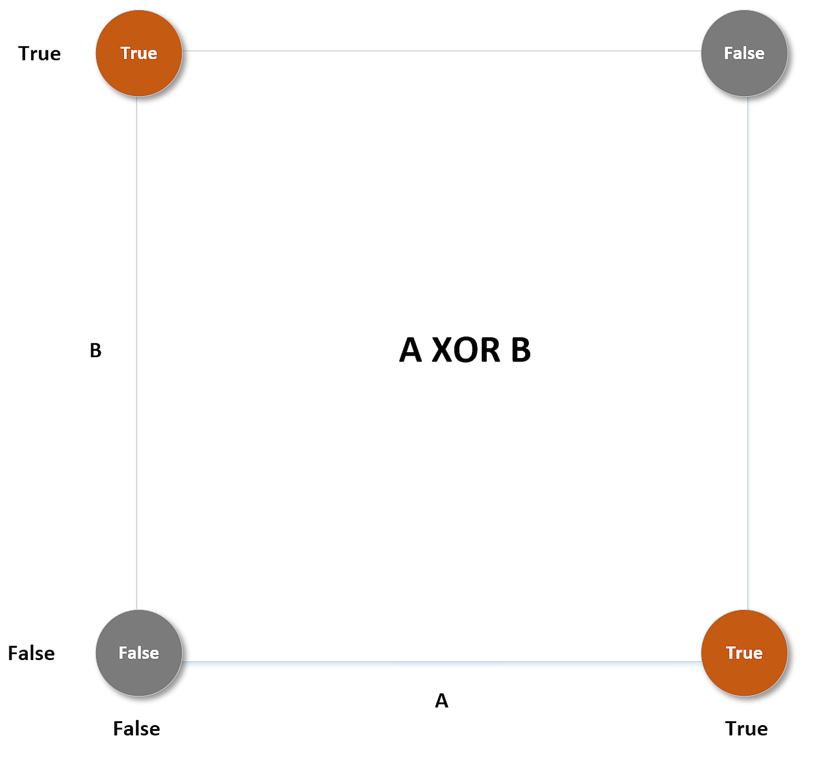
如你所见,不能用直线将True和False分开,非线性可分的情况应该采用非线性计数。
5.2 Logistic regression逻辑回归
Even if called regression, this is a classification method which is based on the probability for a sample to belong to a class. As our probabilities must be continuous in R and bounded between (0, 1), it's necessary to introduce a threshold function to filter the term z. The name logistic comes from the decision to use the sigmoid (or logistic) function:尽管称为回归,这其实是一种基于样本属于某个类的概率的分类方法。由于概率在实数R中是连续的,并且在(0,1)之间有界,所以有必要引入一个阈值函数来过滤z项。logistic这个名称是因为使用sigmoid(或logistic)函数:

$$\sigma(z)=\frac{1}{1+e^{-z}} \ which \ becomes \ \sigma(\vec{x};\vec{w})=\frac{1}{1+e^{-\vec{w}^T\cdot\vec{x}}}$$
A partial plot of this function is shown in the following figure:这个函数的部分图如下图所示:
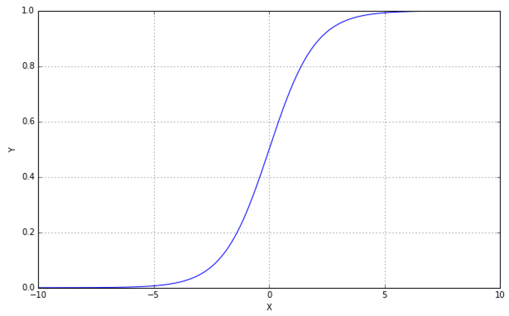 As you can see, the function intersects x=0 in the ordinate 0.5, and y<0.5 for x<0 and y>0.5 for x>0. Moreover, its domain is R and it has two asymptotes at 0 and 1. So, we can define the probability for a sample to belong to a class (from now on, we'll call them 0 and 1) as:如您所见,函数与x=0相交于纵坐标0.5,y<0.5为x<0, y>0.5为x>0。而且,它的定义域是实数R且它有两个渐近线分别渐进到0和1。因此,我们可以定义样本属于一个类的概率(从现在开始,我们称它们为0和1):

$$P(y|\vec{x})=\sigma(\vec{x};\vec{w})$$
At this point, finding the optimal parameters is equivalent to maximizing the log-likelihood given the output class:在这一点上,找到最优参数等价于最大化给定输出类的对数似然:

$$\log{L(\vec{w};y)}=\log{P(y|\vec{x})}=\sum_{i=1}^{n}{\log{P(y_i|\vec{x}_i,\vec{w})}}$$
Therefore, the optimization problem can be expressed, using the indicator notation, as the minimization of the loss function:因此,优化问题可以用指标表示法表示为损失函数的最小化:

$$J(\vec{w})=-\sum_{i=1}^{n}{\log{P(y_i|\vec{x}_i,\vec{w})}}=-\sum_{i=1}^{n}{(y_i\log{\sigma(z_i)}+(1-y_i)\log{(1-\sigma(z_i))})}$$
【
假设sigmoid函数$\phi{(z_i)}$表示属于1类的概率,于是做出如下的定义:
$$\left\{ \begin{aligned} p(y_i=1|\vec{x}_i) & = \phi{(\vec{w}^T \cdot \vec{x}_i +b)}=\phi{(z_i)} \\ p(y_i=0|\vec{x}_i) & = 1-\phi{(z_i)} \end{aligned} \right.$$
将两个式子综合来,可以改写为下式:
$$p(y_i|\vec{x}_i) = {\hat{y}_i}^{y_i}{(1-\hat{y}_i)}^{(1-y_i)}$$
因为$y_i \in \{0,1\}$;当$y_i=0$时,上式退化为$p(y_i|\vec{x}_i) = {(1-\hat{y}_i)}$;当$y_i=1$时,上式退化为$p(y_i|\vec{x}_i) = {\hat{y}_i}$。
再对上式取对数。 详情见另一篇博文逻辑回归logistic_regression 】
If $y_i=0$, the first term becomes null and the second one becomes log(1-x), which is the log-probability of the class 0. On the other hand, if y=1, the second term is 0 and the first one represents the log-probability of x. In this way, both cases are embedded in a single expression. In terms of information theory, it means minimizing the cross-entropy between a target distribution and an approximated one:如果$y_i=0$,第一项为空,第二项为$\log (1 - \sigma (z_i))$(作者原文表述有误),这是0类的对数概率。另一方面,如果$y_i=1$,第二项是0,第一项代表1类的对数概率。这样,两种情况都嵌入到一个表达式中。从信息论的角度来说,它意味着最小化目标分布和近似分布之间的交叉熵:

$$H(X)=-\sum_{x \in X}{p(x)\log_{2}{q(x)}}$$
In particular, if $log_2$ is adopted, the functional expresses the number of extra bits requested to encode the original distribution with the predicted one. It's obvious that when $J(\vec{w}) = 0$, the two distributions are equal. Therefore, minimizing the cross-entropy is an elegant way to optimize the prediction error when the target distributions are categorical.特别地,如果采用$log_2$,函数就表示用预测的分布编码原始分布所需的额外比特数。显然,当$J(\vec{w}) = 0$时,两个分布相等。因此,当目标分布是分类时,使交叉熵最小是优化预测误差的一种理想方法。
5.3 Implementation and optimizations实现和优化
Let's consider a toy dataset made of 500 samples:考虑一个由500个样本组成的玩具数据集
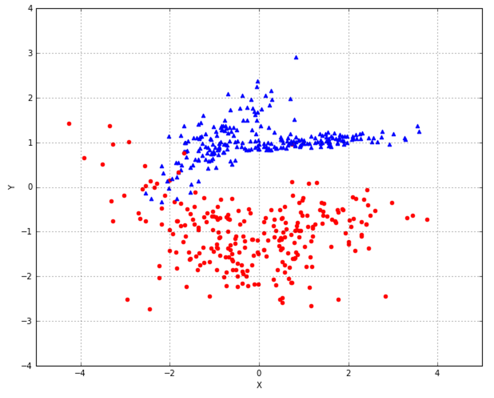 In the following figure, there's a representation of this hyperplane (a line), where it's possible to see how the classification works and what samples are misclassified. Considering the local density of the two blocks, it's easy to see that the misclassifications happened for outliers and for some borderline samples. The latter can be controlled by adjusting the hyperparameters, even if a trade-off is often necessary. For example, if we want to include the four right dots on the separation line, this could exclude some elements in the right part. Later on, we're going to see how to find the optimal solution. However, when a linear classifier can easily find a separating hyperplane (even with a few outliers), we can say that the problem is linearly modelable; otherwise, more sophisticated non-linear techniques must be taken into account.在下面的图中,有一个超平面(直线)的表示,可以看到分类是如何工作的,以及哪些样本被错误分类。考虑到这两个块的局部密度,很容易看到异常值和一些边缘样本的误分类。后者可以通过调整超参数来控制,即使经常需要权衡取舍。例如,如果我们想在分离线上包含右边四个点,这可能会排除右边部分的一些元素。稍后,我们将看到如何找到最优解。然而,当一个线性分类器可以很容易地找到一个分离超平面(即使有一些离群值),我们可以说这个问题是线性可建模的;否则,必须考虑更复杂的非线性技术。
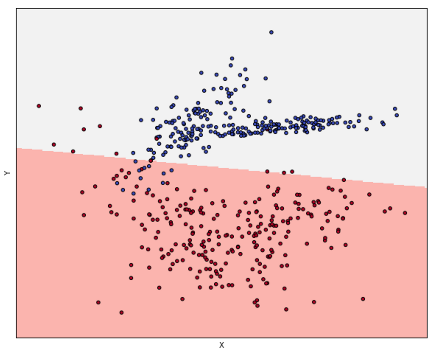 Just like for linear regression, it's possible to impose norm conditions on the weights. In particular, the actual functional becomes: 就像线性回归一样,可以对权值施加范数条件。具体来说,实际的函数为:

$$\hat{J}(\vec{w})=\left\{ \begin{aligned} J(\vec{w})+\alpha\|\vec{w}\|_1 \\ J(\vec{w})+\alpha\|\vec{w}\|_2^2 \end{aligned} \right.$$
The behavior is the same as explained in the previous chapter. Both produce a shrinkage, but L1 forces sparsity.行为与在前面一章中一样,都能产生参数收缩,而且L1强制参数稀疏。
5.4 Stochastic gradient descent algorithms随机梯度下降算法
It's useful to introduce the SGDClassifier class , which implements a very famous algorithm that can be applied to several different loss functions. The idea behind stochastic gradient descent is iterating a weight update based on the gradient of loss function: 引入SGDClassifier类是很有用的,它实现了一个非常著名的算法,可以应用于几个不同的损失函数。随机梯度下降的思想是迭代一个基于损失函数梯度的权值更新:

$$\vec{w}(k+1)=\vec{w}(k)-\gamma\nabla{L(\vec{w})}$$
However, instead of considering the whole dataset, the update procedure is applied on batches randomly extracted from it. In the preceding formula, $L$ is the loss function we want to minimize (as discussed in Chapter 2, Important Elements in Machine Learning) and gamma (eta0 in scikit-learn) is the learning rate, a parameter that can be constant or decayed while the learning process proceeds. The learning_rate parameter can be also left with its default value (optimal), which is computed internally according to the regularization factor.然而,更新过程并没有考虑整个数据集,而是对随机提取的批进行更新。在前面的公式中,$L$是我们想要最小化的损失函数(如第2章“机器学习中的重要元素”所讨论的那样),而gamma (scikit-learn中的eta0)是学习率,在学习过程中,这个参数可以是常数,也可以是衰减的。learning_rate参数还可以保留其默认值(最优值),该值根据正则化因子在内部计算。
The process should end when the weights stop modifying or their variation keeps itself under a selected threshold. The scikit-learn implementation uses the n_iter parameter to define the number of desired iterations.当权值停止修改或其变化保持在一个选定的阈值下时,该过程应该结束。scikit-learn实现使用n_iter参数来定义所需的迭代次数。
There are many possible loss functions, but in this chapter, we consider only log and perceptron. Some of the other ones will be discussed in the next chapters. The former implements a logistic regression, while the latter (which is also available as the autonomous class Perceptron) is the simplest neural network, composed of a single layer of weights w, a fixed constant called bias, and a binary output function: (SGDClassifier)有许多可能的损失函数,但在本章中,我们只考虑log和perceptron(即逻辑回归和感知器)。其他一些将在下一章中讨论。前者实现逻辑回归,而后者(也可作为自主类感知器使用)是最简单的神经网络,由一层权重$\vec{w}$、一个称为偏差的固定常数和一个二进制输出函数组成:
The output function (which classifies in two classes) is:输出函数(分类为两个类)是:
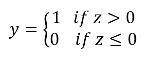
$$f(n) = \begin{cases} 1, & \text{if $z \ge 0$} \\ 0, & \text{if $z \le 0$} \end{cases}$$

$$z=\vec{w}^T\cdot\vec{x}+b$$
The differences between a Perceptron and a LogisticRegression are the output function (sign versus sigmoid) and the training model (with the loss function). A perceptron, in fact, is normally trained by minimizing the mean square distance between the actual value and prediction: Perceptron和LogisticRegression的区别在于输出函数(符号对sigmoid)和训练模型(损失函数)。实际上,感知器通常是通过最小化实际值和预测之间的均方距离来训练的:
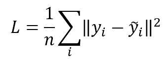
$$L=\frac{1}{n}\sum_{i=1}^{n}{\|y_i-\hat{y}_i\|_2^2}$$
Just like any other linear classifier, a perceptron is not able to solve nonlinear problems; hence, our example will be generated using the built-in function make_classification:就像其他线性分类器一样,感知器不能解决非线性问题;因此,我们的示例将使用内置函数make_classification生成:
In this way, we can generate 500 samples split into two classes:这样,我们可以生成分成两个类的500个样本
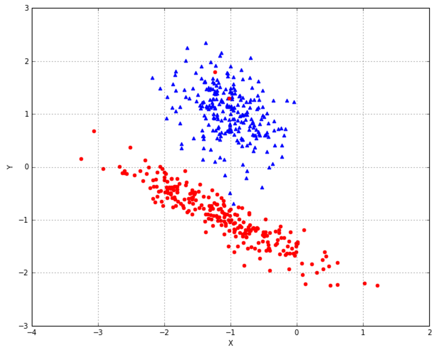 This problem, under a determined precision threshold, can be linearly solved, so our expectations are equivalent for both
 Perceptron and LogisticRegression. In the latter case, the training strategy is focused on maximizing the likelihood of a probability distribution. Considering the dataset, the probability of a red sample to belong to class 0 must be greater than 0.5 (it's equal to 0.5 when z = 0, so when the point lays on the separating hyperplane) and vice versa. On the other hand, a perceptron will adjust the hyperplane so that the dot product between a sample and the weights would be positive or negative, according to the class. In the following figure, there's a geometrical representation of a perceptron (where the bias is 0):这个问题,在一个确定的精度阈值下,可以线性地解决,所以我们对Perceptron和LogisticRegression的期望是相等的。在后一种情况下,训练策略集中于最大化概率分布的似然。考虑到数据集,一个红色样本属于0类的概率必须大于0.5(所以当点位于分离超平面上时,当z=0时红色样本属于0类的概率等于0.5),反之亦然。另一方面,根据分类,感知器会调整超平面,使样本和权值之间的点积为正或负。在下面的图中,有一个感知器的几何表示(偏差为0):
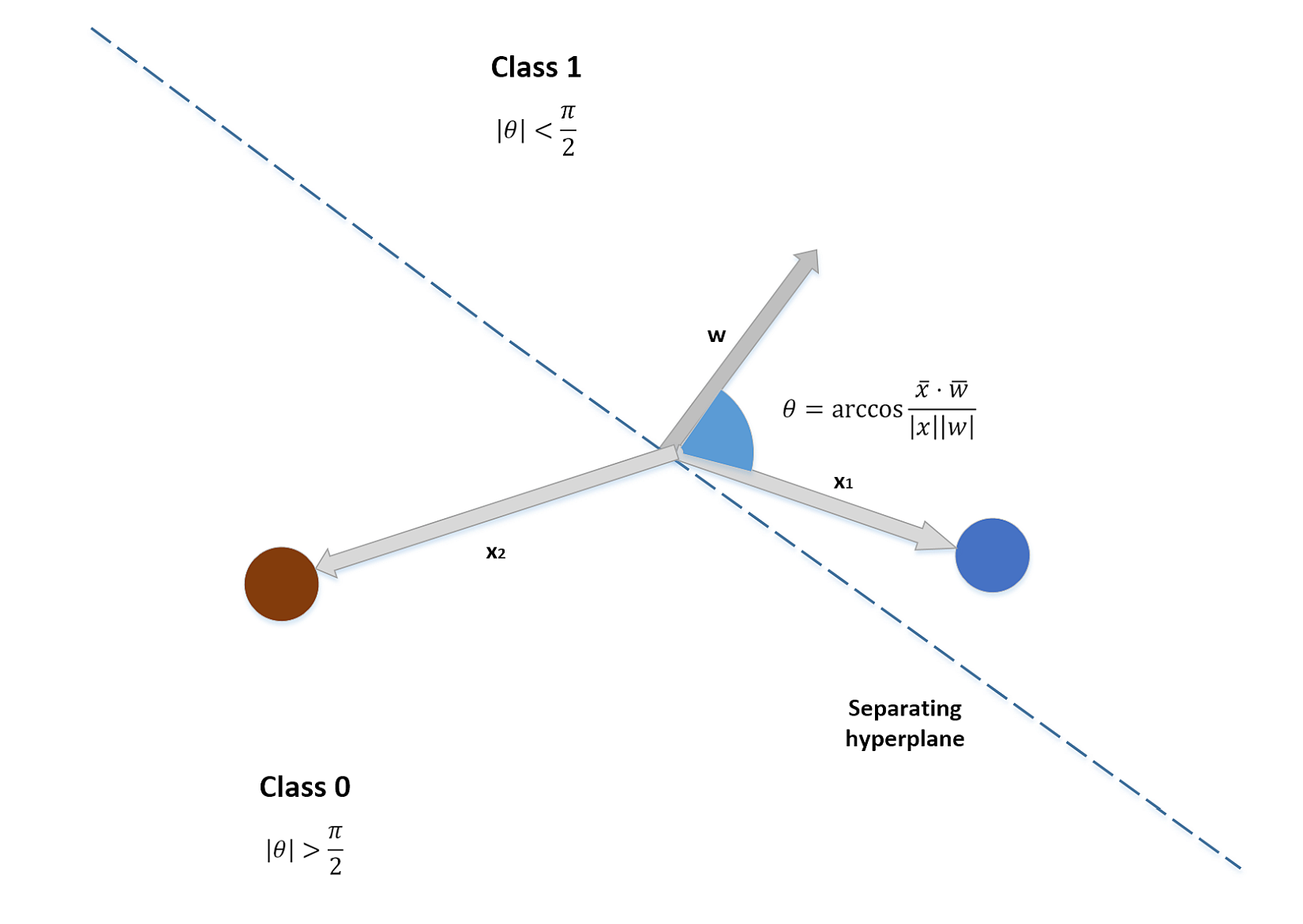 The weight vector is orthogonal to the separating hyperplane, so that the discrimination can happen only considering the sign of the dot product.权向量与分离超平面正交,因此只考虑点积的符号就可以进行鉴别(鉴别分类)。
感知器通常采用MSE,但分类问题若采用MSE损失函数,其损失函数将不是凸函数,优化时候易于陷入局部最优。所以sklearn之LogisticRegression仅支持log损失函数,LogisticRegression采用log损失函数是凸函数。sklearn之SGDClassifier可以选择MSE,随机梯度下降SGD可避免陷于局部优化。可以阅读逻辑回归logistic_regression。
5.5 Finding the optimal hyperparameters through grid search通过网格搜索寻找最优高参
In the next example, we're going to find the best parameters of an SGDClassifier trained with perceptron loss. The dataset is plotted in the following figure:在下一个例子中,我们将找到SGDClassifier采用感知器损失训练的最佳参数。数据集作图如下:
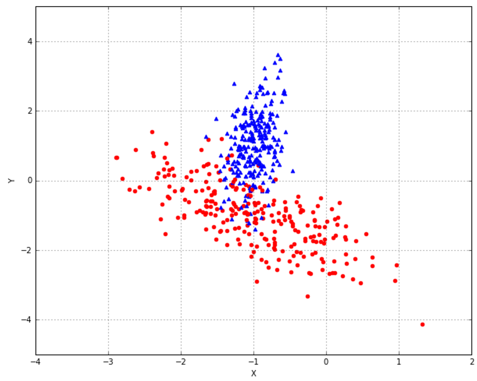 网格搜索在sklearn中有
GridSearchCV,甚至可被keras调用,很简单,略。
5.6 Classification metrics分类度量尺度
A classification task can be evaluated in many different ways to achieve specific objectives. Of course, the most important metric is the accuracy, often expressed as:分类任务可以用许多不同的方式进行评估,以实现特定的目标。当然,最重要的度量标准是精确度,通常表示为:

$$\text{Generic accuracy}=1-\frac{\text{Number of misclassified samples}}{\text{Total number of samples}}$$
Another very common approach is based on zero-one loss function, which we saw in Chapter 2, Important Elements in Machine Learning, which is defined as the normalized average of L0/1 (where 1 is assigned to misclassifications) over all samples.另一通常方法是基于0-1损失函数,第二章出现过,这个方法定义为所有样本的归一化平均L0/1(其中1被分配给误分类)。(对于二分类,值与精确度和为1)。
A similar but opposite metric is the Jaccard similarity coefficient, defined as:另一个相似但相反的度量是Jaccard相似系数,定义为:
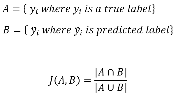
$$A=\{y_i \ where \ y_i \text{ is a true label}\}\\
B=\{\hat{y}_i \ where \ \hat{y}_i \text{ is a true label}\}\\
J(A,B)=\frac{|A \cap B|}{|A \cup B|}$$
看定义,其实就是判断正确的数量与总样本数的比值,结果与精确度相同,与0-1损失和为1。
These measures provide a good insight into our classification algorithms. However, in many cases, it's necessary to be able to differentiate between different kinds of misclassifications (we're considering the binary case with the conventional notation: 0-negative, 1-positive), because the relative weight is quite different. For this reason, we introduce the following definitions:这些测量为我们的分类算法提供了一个很好的视角。然而,在许多情况下,有必要区分不同类型的误分类(我们考虑的是传统符号即0-负、1-正的二进制情况),因为相对权重非常不同。因此,引入下列定义:
- True positive: A positive sample correctly classified 真阳性: 阳性样本被划分为阳性
- False positive: A negative sample classified as positive 假阳性: 阴性样本被划分为阳性
- True negative: A negative sample correctly classified 真阴性: 阴性样本被划分为阴性
- False negative: A positive sample classified as negative 假阴性: 阳性样本被划分为阴性
At a glance, false positive and false negative can be considered as similar errors, but think about a medical prediction: while a false positive can be easily discovered with further tests, a false negative is often neglected, with repercussions following the consequences of this action. For this reason, it's useful to introduce the concept of a confusion matrix:乍一看,假阳性和假阴性可以被认为是类似的错误,但想想一个医学预测:一个假阳性很容易通过进一步的测试发现,一个假阴性往往被忽视,这一行动将产生后果。因此,引入混淆矩阵的概念是很有用的:
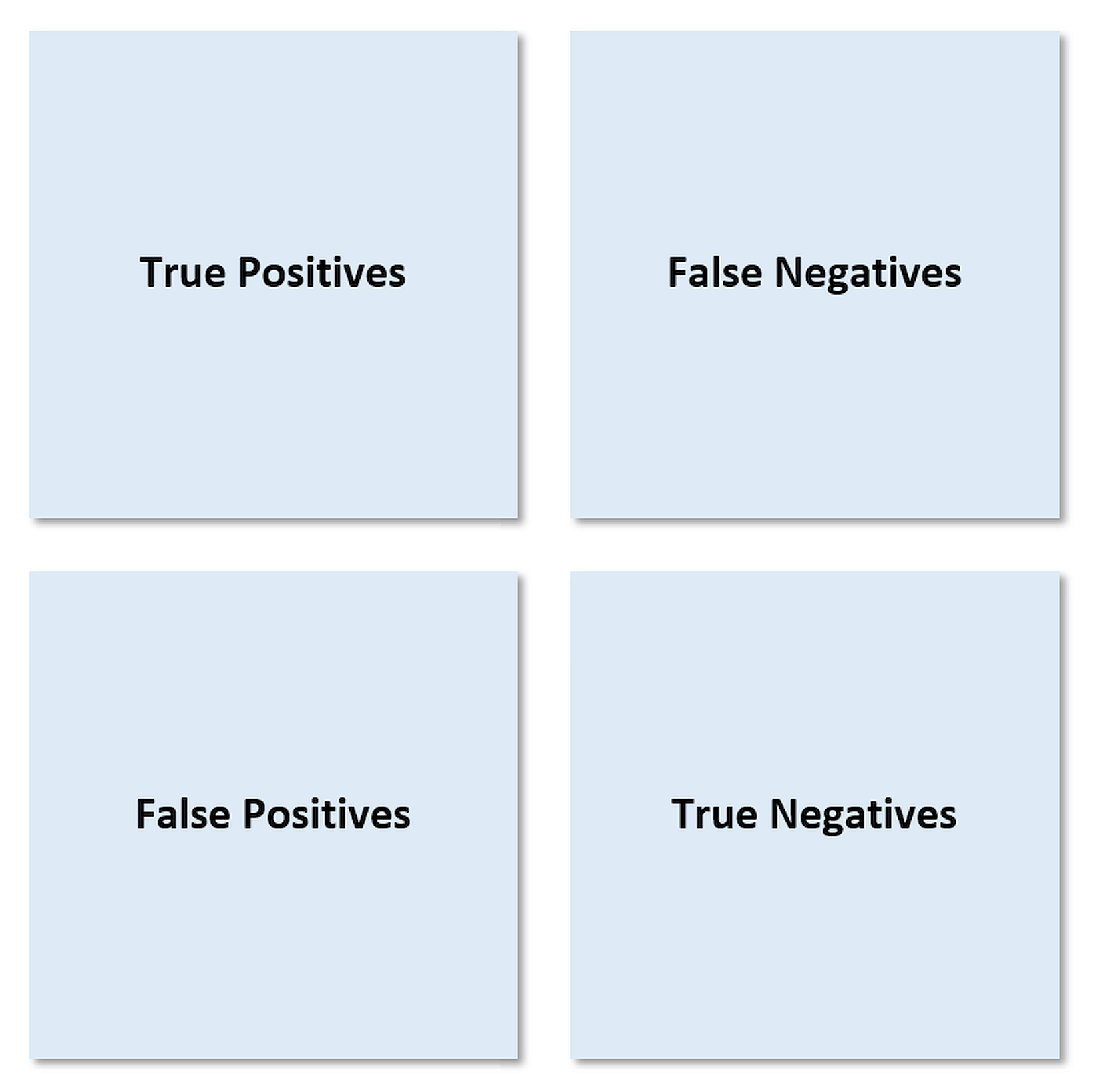 So we have five false negatives and two false positives. If needed, a further analysis can allow for the detection of the misclassifications to decide how to treat them (for example, if their variance overcomes a predefined threshold, it's possible to consider them as outliers and remove them).因此如果我们有5个假阴性和2个假阳性。如果需要,进一步的分析可以检测错误分类以决定如何处理它们(例如,如果它们的方差超过预定义的阈值,则可以将它们视为离群值并删除它们)。
Another useful direct measure is:另一个有用的直接度量是:

$$\text{Precision}=\frac{\text{True positives}}{\text{True positives}+\text{False positives}}$$
This is directly connected with the ability to capture the features that determine the positiveness of a sample, to avoid the misclassification as negative.这与捕获特征以确定阳性样本的能力直接相关,以避免误分类为阴性。
The ability to detect true positive samples among all the potential positives can be assessed using another measure:在所有潜在的阳性样本中检测出真正阳性样本的能力可以用另一种方法来评估:

$$\text{Recall}=\frac{\text{True positives}}{\text{True positives}+\text{False negatives}}$$
It's not surprising that we have a 90 percent recall with 96 percent precision, because the number of false negatives (which impact recall) is proportionally higher than the number of false positives (which impact precision). A weighted harmonic mean between precision and recall is provided by:我们有90%的召回率,准确率为96%,这并不奇怪,因为假阴性的数量(影响召回率)比假阳性的数量(影响精度)成比例的高。精度与查全之间的加权调和均值如下:

$$F_{Beta}=({\beta}^2+1)\frac{\text{Precision}\cdot\text{Recall}}{({\beta}^2\text{Precision})+\text{Recall}}$$
A beta value equal to 1 determines the so-called F1 score, which is a perfect balance between the two measures. A beta less than 1 gives more importance to precision and a value greater than 1 gives more importance to recall. beta等于1决定了所谓的F1分数,这是两项指标之间的完美平衡。beta小于1更注重准确率,beta大于1注重召回率。
5.7 ROC curve ROC曲线
The ROC curve (or receiver operating characteristics) is a valuable tool to compare different classifiers that can assign a score to their predictions. In general, this score can be interpreted as a probability, so it's bounded between 0 and 1. The plane is structured like in the following figure:ROC曲线(或接收器工作特性)是比较不同的分类器的一个有价值的工具,这些分类器可以为它们的预测打分。一般来说,这个分数可以解释为概率,所以它在0和1之间有界。它的界在0和1之间。平面的结构如下图所示:
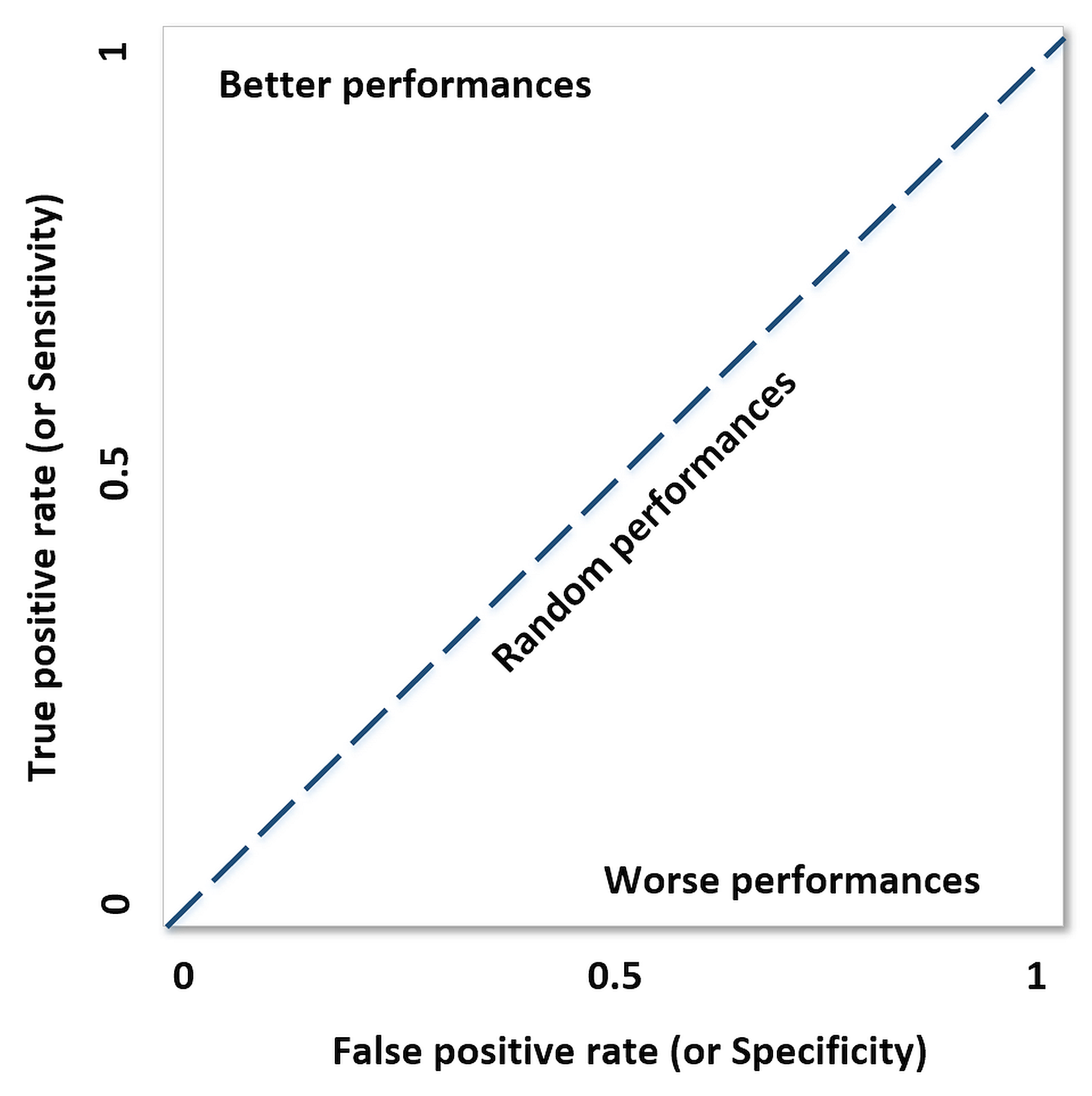 The x axis represents the increasing false positive rate (also known as specificity), while the y axis represents the true positive rate (also known as sensitivity). The dashed oblique line represents a perfectly random classifier, so all the curves below this threshold perform worse than a random choice, while the ones above it show better performances. Of course, the best classifier has an ROC curve split into the segments [0, 0] - [0, 1] and [0, 1] - [1, 1], and our goal is to find algorithms whose performances should be as close as possible to this limit. x轴表示错正率增加(也称为特异性),y轴表示对正率(也称为敏感性)。虚线斜线表示一个完全随机的分类器,因此低于这个阈值的所有曲线都比随机选择的差,而高于这个阈值的曲线表现更好。当然,最好的分类器有一个分割为[0,0]-[0,1]和[0,1]-[1,1]片段的ROC曲线,我们的目标是找到性能应该尽可能接近这个极限的算法。
Before proceeding, it's also useful to compute the area under the curve (AUC), whose value is bounded between 0 (worst performances) and 1 (best performances), with a perfectly random value corresponding to 0.5:在继续之前,还需要计算曲线下的面积(AUC),其值在0(最差性能)和1(最佳性能)之间有界,其完全随机值对应于0.5:
The resulting ROC curve is the following plot:得到的ROC曲线如下图所示:
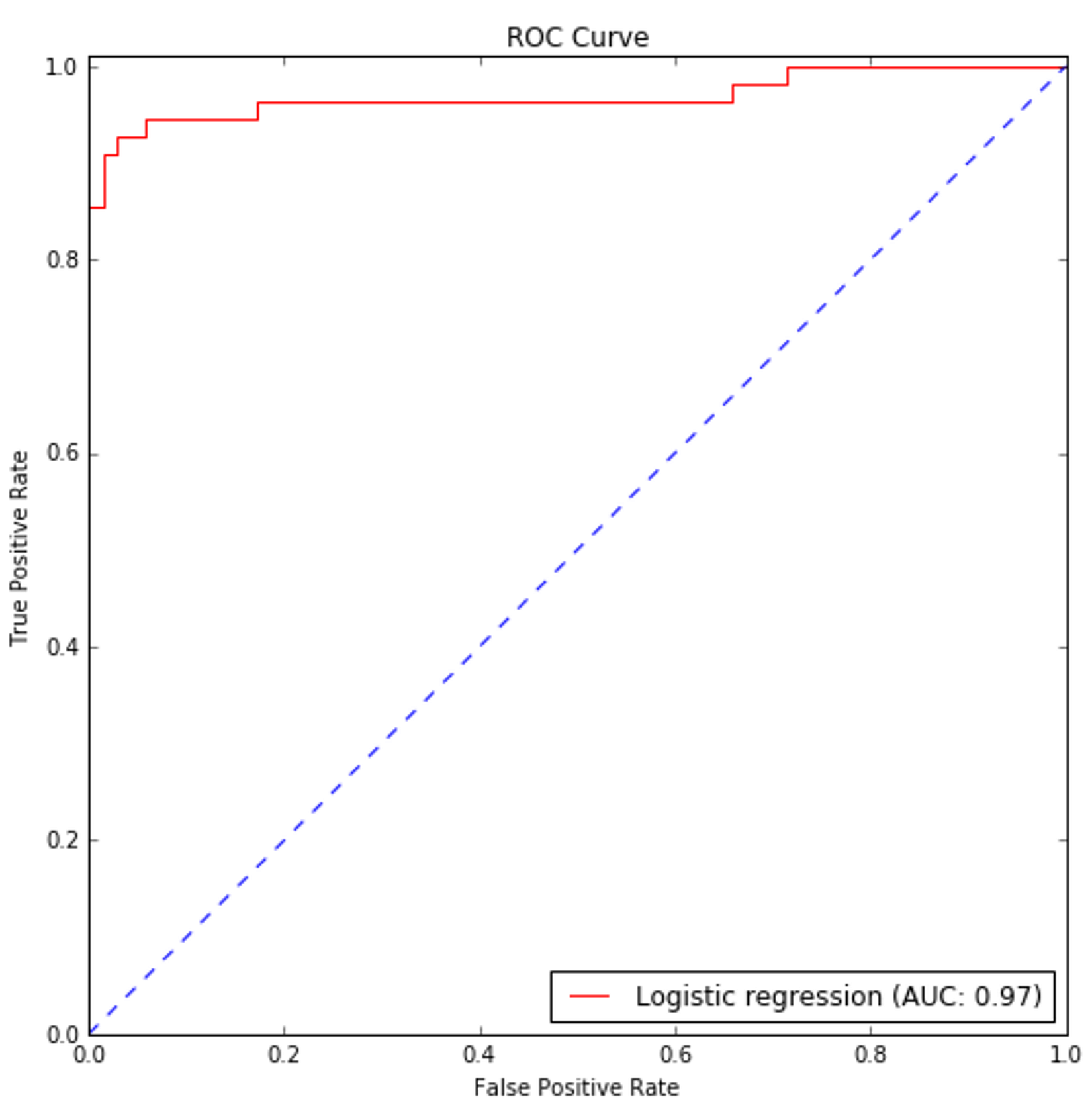 datetime 2018//11/22 15:08
5.8 Summary总结
6 Naive Bayes朴素贝叶斯
Naive Bayes are a family of powerful and easy-to-train classifiers that determine the probability of an outcome given a set of conditions using Bayes' theorem. In other words, the conditional probabilities are inverted, so that the query can be expressed as a function of measurable quantities. The approach is simple, and the adjective "naive" has been attributed not because these algorithms are limited or less efficient, but because of a fundamental assumption about the causal factors that we're going to discuss. Naive Bayes are multi-purpose classifiers and it's easy to find their application in many different contexts; however, their performance is particularly good in all those situations where the probability of a class is determined by the probabilities of some causal factors. A good example is natural language processing, where a piece of text can be considered as a particular instance of a dictionary and the relative frequencies of all terms provide enough information to infer a belonging class. 朴素贝叶斯是一个强大且易于训练的分类器家族,它使用贝叶斯定理在给定一组条件下确定结果的概率。换句话说,条件概率是反向的,这样查询就可以表示为可测量量的函数。这个方法很简单,形容词“朴素”之所以被归为“朴素”,并不是因为这些算法有限或效率较低,而是因为我们将要讨论的一个关于因果因素的基本假设。朴素贝叶斯是一种多用途的分类器,很容易在许多不同的语境中找到它们的应用;然而,在所有这些情况下,它们的性能都特别好,因为类的概率是由一些因果因素的概率决定的。一个很好的例子是自然语言处理,其中一段文本可以被看作是字典的一个特定实例,所有术语的相对频率提供了足够的信息来推断属于哪个类。
6.1 Bayes' theorem贝叶斯理论
Let's consider two probabilistic events A and B. We can correlate the marginal probabilities P(A) and P(B) with the conditional probabilities P(A|B) and P(B|A) using the product rule:让我们考虑两个概率事件A和B。我们可以用乘积法则将边际概率P(A)和P(B)与条件概率P(A|B)和P(B|A)联系起来:

$$\left\{ \begin{aligned} P(A \cap B) & = P(A \mid B)P(B) \\ P(B \cap A) & = P(B \mid A)P(A) \end{aligned} \right.$$
Considering that the intersection is commutative, the first members are equal; so we can derive Bayes' theorem:考虑到交集是可交换的,第一部分是相等的;我们可以推导出贝叶斯定理:

$$P(A \mid B)=\frac{P(B \mid A)P(A)}{P(B)}$$
This formula has very deep philosophical implications and it's a fundamental element of statistical learning. First of all, let's consider the marginal probability P(A); this is normally a value that determines how probable a target event is, such as P(Spam) or P(Rain). As there are no other elements, this kind of probability is called Apriori, because it's often determined by mathematical considerations or simply by a frequency count. For example, imagine we want to implement a very simple spam filter and we've collected 100 emails. We know that 30 are spam and 70 are regular. So we can say that P(Spam) = 0.3.这个公式有很深的哲学含义,是统计学习的基本要素。首先考虑边际概率P(A),这通常是一个确定目标事件的可能性的值,例如P(Spam)或P(Rain)。由于没有其他元素,这种概率被称为先验概率,因为它通常由数学考虑或简单的频率计数决定。例如,假设我们要实现一个非常简单的垃圾邮件过滤器,我们已经收集了100封电子邮件。我们知道30是垃圾邮件,70是常规邮件。所以可以说P(Spam)=0.3。
However, we'd like to evaluate using some criteria (for simplicity, let's consider a single one), for example, email text is shorter than 50 characters. Therefore, our query becomes:但是,我们希望使用一些标准来评估(为了简单起见,让我们考虑一个),例如,电子邮件文本小于50个字符。因此,我们的查询变成:

$$P({Spam} \mid {Text}<50 \ {Chars})=\frac{P({Text}<50 \ {Chars} \mid {Spam})P({Spam})}{P({Text}<50 \ {Chars})}$$
The first term is similar to P(Spam) because it's the probability of spam given a certain condition. For this reason, it's called a posteriori (in other words, it's a probability that we can estimate after knowing some additional elements). On the right-hand side, we need to calculate the missing values, but it's simple. Let's suppose that 35 emails have text shorter than 50 characters, so P(Text < 50 chars) = 0.35. Looking only into our spam folder, we discover that only 25 spam emails have short text, so that P(Text < 50 chars|Spam) = 25/30 = 0.83. The result is:第一项类似于P(Spam),因为它是特定条件下垃圾邮件发生的概率。因此,它被称为后验概率(换句话说,它是我们在知道一些额外的元素后可以估计的概率)。另外,我们需要计算缺失值,但很简单。假设35封电子邮件的文本长度小于50个字符,那么P(Text<50 chars)= 0.35。只看垃圾邮件箱,发现只有25封邮件文本长度短,因此P(Text < 50 chars|Spam) = 25/30 = 0.83。结果如下:

$$P({Spam} \mid {Text}<50 \ {Chars})=\frac{0.83 \cdot 0.3}{0.35}=0.71$$
So, after receiving a very short email, there is a 71% probability that it's spam. Now, we can understand the role of P(Text < 50 chars|Spam); as we have actual data, we can measure how probable is our hypothesis given the query. In other words, we have defined a likelihood (compare this with logistic regression), which is a weight between the Apriori probability and the a posteriori one (the term in the denominator is less important because it works as a normalizing factor):所以,在收到一封很短的电子邮件后,71%的概率是垃圾邮件。现在,我们可以理解P(Text < 50 chars|Spam)的角色;由于我们有实际的数据,我们可以测量在查询下我们的假设的可能性有多大。换句话说,我们定义了一种似然(与logistic回归相比),它是先验概率和后验概率之间的权重(分母中的术语不那么重要,因为它是一个标准化因子):

$$P_{A-Posteriori}\propto {Likelihood} \cdot P_{A-Priori}$$
The normalization factor is often represented by the Greek letter alpha, so the formula becomes:标准化因子通常用希腊字母表示,所以公式变成:

$$P(A \mid B)=\alpha P(B \mid A)P(A)$$
The last step is considering the case when there are more concurrent conditions (this is more realistic in real-life problems):最后一步是考虑有更多并发条件的情况(这在实际问题中更现实):

$$P(A \mid C_1 \cap C_2 ... \cap C_m)$$
A common assumption is called conditional independence (in other words, the effects produced by every cause are independent of each other) and this allows us to write a simplified expression:一个常见的假设叫做条件独立(换句话说,每个原因产生的结果是相互独立的),这允许我们编写一个简化的表达式:

$$P(A \mid C_1 \cap C_2 ... \cap C_m) = \alpha P(C_1 \mid A) P(C_2 \mid A) ... P(C_m \mid A)$$
【
贝叶斯定理:
$$P(A \mid C_1 \cap C_2 ... \cap C_m) = \alpha P(C_1 \cap C_2 ... \cap C_m \mid A) P(A)$$
条件独立假设:
$$P(C_1 \cap C_2 ... \cap C_m \mid A) = P(C_1 \mid A) P(C_2 \mid A) ... P(C_m \mid A)$$
那么上式得证。
作者用n,被我改成m,因为$C_i$其实是一列特征。
】
6.2 Naive Bayes classifiers朴素贝叶斯分类器
A naive Bayes classifier is called so because it's based on a naive condition, which implies the conditional independence of causes. This can seem very difficult to accept in many contexts where the probability of a particular feature is strictly correlated to another one. For example, in spam filtering, a text shorter than 50 characters can increase the probability of the presence of an image, or if the domain has been already blacklisted for sending the same spam emails to million users, it's likely to find particular keywords. In other words, the presence of a cause isn't normally independent from the presence of other ones. However, in Zhang H., The Optimality of Naive Bayes, AAAI 1, no. 2 (2004): 3, the author showed that under particular conditions (not so rare to happen), different dependencies clears one another, and a naive Bayes classifier succeeds in achieving very high performances even if its naiveness is violated.朴素贝叶斯分类器之所以被称为朴素贝叶斯分类器,是因为它基于朴素条件,这意味着原因(原因之间,也就是特征之间)的条件独立性。在许多情况下,这似乎很难接受,因为一个特定特性的概率与另一个特性的概率是严格相关的。例如,在垃圾邮件过滤中,少于50个字符的文本可能会增加图像出现的可能性,或者如果该域已经因为向数百万用户发送相同的垃圾邮件而被列入黑名单,那么它很可能会找到特定的关键字。换句话说,一个原因的存在通常并不独立于其他原因的存在。Zhang H文章证明特征即使不条件独立,朴素贝叶斯分类器表现仍然很好。
Let's consider a dataset:让我们考虑一个数据集:

$$\mathbf{X}=\{\vec{x}_1,\vec{x}_2,\ldots,\vec{x}_n\} \ where \ \vec{x}_i \in \mathbb{R}^m$$
Every feature vector, for simplicity, will be represented as:为了简单起见,每个数据点(原文为特征向量,应是作者笔误)向量都表示为:

$$\vec{x}_i = [x_1;x_2;\ldots,x_n]$$
We need also a target dataset:我们还需要一个目标数据集:

$$y=\{y_1,y_2,\ldots,y_n\} \ where \ y_i \in \{1,2,\ldots,P\}$$
Here, each y can belong to one of P different classes. Considering Bayes' theorem under conditional independence, we can write:在这里,每个y都可以属于P个不同的类之一。考虑条件独立性下的贝叶斯定理,我们可以这样写:

$$P(y \mid x_1,x_2,\ldots,x_m) = \alpha P(y)\prod_{i=1}^{m}{P(x_i \mid y)}$$
这里$x_1,\ldots,x_m$是一行数据,这m个数构成一个行向量$[x_1,x_2,\ldots,x_m]$。
The values of the marginal Apriori probability P(y) and of the conditional probabilities P(xi|y) is obtained through a frequency count; therefore, given an input vector x, the predicted class is the one for which the a posteriori probability is maximum.通过频率计数得到了边际先验概率P(y)和条件概率P(xi|y)的值;因此,给定一个输入向量x,预测类就是后验概率最大的类。
6.3 Naive Bayes in scikit-learn scikit-learn中的朴素贝叶斯
scikit-learn implements three naive Bayes variants based on the same number of different probabilistic distributions: Bernoulli, multinomial, and Gaussian. The first one is a binary distribution, useful when a feature can be present or absent. The second one is a discrete distribution and is used whenever a feature must be represented by a whole number (for example, in natural language processing, it can be the frequency of a term), while the third is a continuous distribution characterized by its mean and variance. scikit-learn实现了三个朴素贝叶斯变体,它们基于相同数量的不同概率分布:伯努利分布、多项式分布和高斯分布。第一种(BernoulliNB)是特征二分分布,在(每个)特征可能出现或不出现(即每个特征是二分的)时非常有用。第二种(MultinomialNB、ComplementNB)分布是离散分布,当一个特征必须用离散数(原文是说特征必须是整数,但接下来又说可以是频率,显然出现了笔误,作者想表达的其实是特征需是离散数)表示时(例如,在自然语言处理中,它可以是一个词语的频率),第三种(GaussianNB)分布是连续分布,以其均值和方差定义。
| naive Bayes variants | X | Y | depend on |
|---|---|---|---|
| BernoulliNB | 1.n_features>=1; 2.each feature is binary/boolean(continuous variables need to set binarized); 3.each feature is Bernoulli-distributed. |
n_classes>=2 | 1.Bayes theorem; 2.conditional independence; 3.each feature is Bernoulli-distributed. |
| MultinomialNB | 1.n_features>=1; 2.each feature is count variable(However, in practice, fractional counts such as tf-idf may also work); 3.each feature is Multinomial-distributed. |
n_classes>=2 | 1.Bayes theorem; 2.conditional independence; 3.each feature is Multinomial-distributed. |
| ComplementNB | 1.n_features>=1; 2.each feature is count variable; 3.not all the features are Multinomial-distributed(imbalanced data set). |
n_classes>=2 | 1.Bayes theorem; 2.conditional independence; 3.not all the features are Multinomial-distributed, so need to correct Systemic Errors. |
| GaussianNB | 1.n_features>=1; 2.each feature is continuous variable; 3.Gaussian-distributed. |
1.n_classes>=2 | 1.Bayes theorem; 2.conditional independence; 3.each feature: Gaussian-distributed. |
更详细原理叙述,可阅读我的博文朴素贝叶斯naive_bayes。
6.3.1 Bernoulli naive Bayes伯努利朴素贝叶斯
If $x_j$ is random variable and is Bernoulli-distributed, it can assume only two values (for simplicity, let's call them 0 and 1) and their probability is:如果$x_j$是随机变量,并且是伯努利分布,它只能有两个值(为简便,称其为0和1)(sklearn中BernoulliNB允许数据含有多列。$n \times m$数据矩阵有$m$列,$x_j$是其中第$j$列,这里将其视作一个伯努利分布的变量。),两个值的概率是:
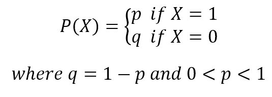
$$P(x_j) = \begin{cases} p, & \text{if $x_j=1$} \\ q, & \text{if $x_j=0$} \end{cases}  \\
\text{where $q = 1 - p$ and $0 < p < 1$}$$
To try this algorithm with scikit-learn, we're going to generate a dummy dataset. Bernoulli naive Bayes expects binary feature vectors; however, the class BernoulliNB has a binarize parameter, which allows us to specify a threshold that will be used internally to transform the features:为了用scikit-learn来尝试这个算法,我们将生成一个虚拟数据集。伯努利朴素贝叶斯期望二元特征向量;然而,BernoulliNB类有一个binarize参数,它允许我们指定一个阈值,该阈值将在内部用于转换特性(将非二分特征转化为二分特征):
We have generated the bidimensional dataset shown in the following figure:我们已经生成了如下图所示的二维数据集:
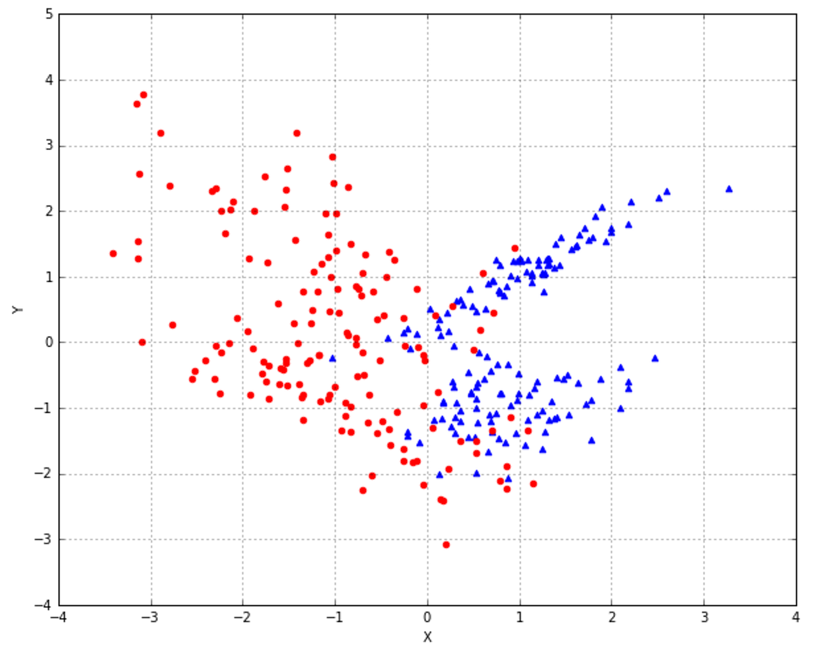 根据书本上的数据生成函数,X为特征,Y为目标。n_features=2说明有两个特征,那么上图该用
$x_1$、$x_2$。两种颜色代表只有两个分类,但注意,伯努利朴素贝叶斯目标是分类,并不要求目标只有两个分类。
若特征连续,binarize取值将显著影响分类效果。但binarize是不可学习的,需网格搜索此高参的合适值。
We have decided to use 0.0 as a binary threshold, so each point can be characterized by the quadrant where it's located. Of course, this is a rational choice for our dataset, but Bernoulli naive Bayes is envisaged for binary feature vectors or continuous values, which can be precisely split with a predefined threshold:我们决定使用0.0作为二进制阈值,这样每个点都可以用它所在的象限来表示。当然,对于我们的数据集来说,这是一个合理的选择,但是伯努利朴素贝叶斯是为二进制特征向量或连续值设想的,连续值可以用预定义的阈值精确分割:
The score is rather good, but if we want to understand how the binary classifier worked, it's useful to see how the data has been internally binarized:分数相当不错,但如果我们想了解二分分类器是如何工作的,那么查看数据是如何内部实现二分化的是很有用的:
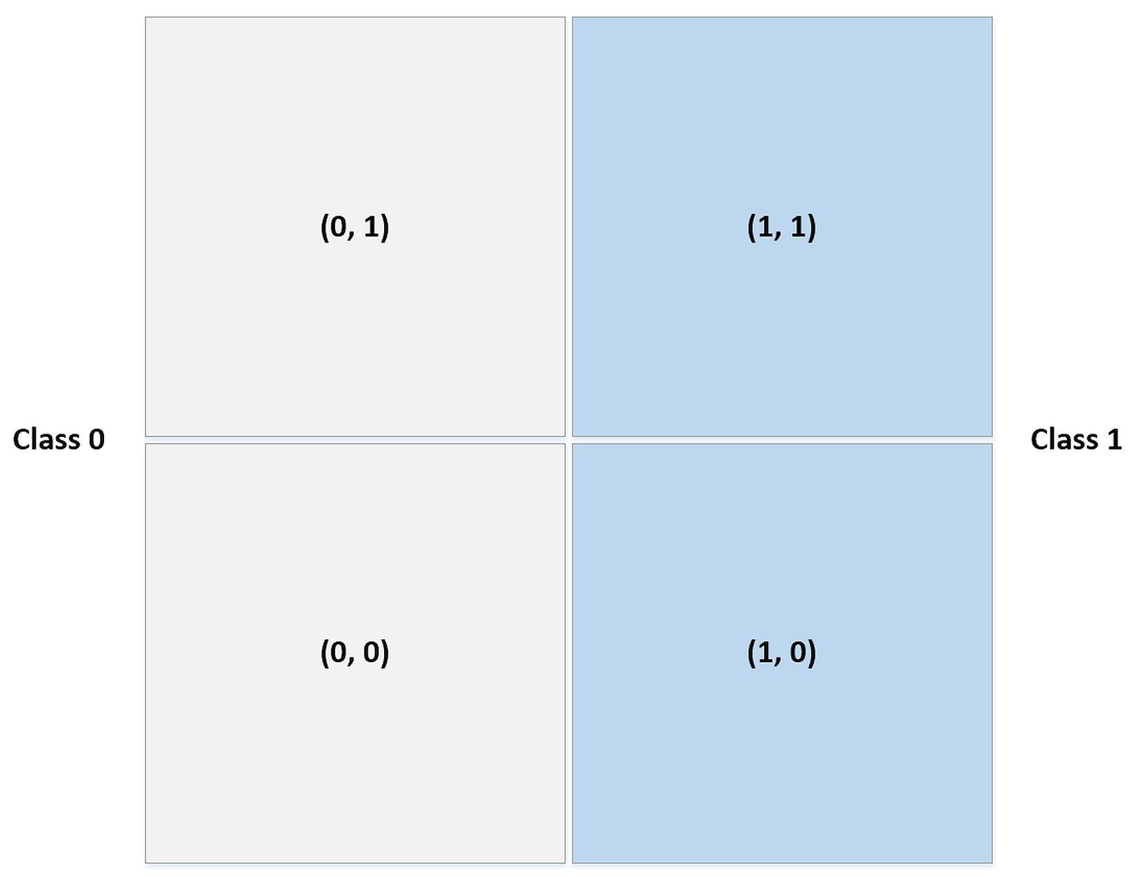
6.3.2 Multinomial naive Bayes多项式朴素贝叶斯
A multinomial distribution is useful to model feature vectors where each value represents, for example, the number of occurrences of a term or its relative frequency. If the feature vectors have $n$ elements and each of them can assume $k$ different values with probability $p_k$, then:多项式分布对于建模特征向量很有用,其中每个值都表示比如一个项的出现次数或一个项的相对频率。如果特征向量有$n$个元素,每个元素假设有$k$个不同的值,每个值的概率是$p_k$,那么:

$$$$
The conditional probabilities $P(x_i|y)$ are computed with a frequency count (which corresponds to applying a maximum likelihood approach), but in this case, it's important to consider the alpha parameter (called Laplace smoothing factor). Its default value is 1.0 and it prevents the model from setting null probabilities when the frequency is zero. It's possible to assign all non-negative values; however, larger values will assign higher probabilities to the missing features and this choice could alter the stability of the model. 条件概率$P(x_i|y)$是用频率计数(对应于应用最大似然方法)来计算的,但在这种情况下,重要的是考虑alpha参数(称为拉普拉斯平滑因子)。它的默认值是1.0,当频率为0时,它阻止模型设置零概率。(alpha)可以分配所有非负值;然而,更大的值会给缺失的特征赋予更高的概率,这种选择可能会改变模型的稳定性。
朴素贝叶斯的特征的分布是理论分布(empirical distribution function )并加了平滑,当然,为了无误确认可能要详读源码了,暂略。可阅读我的博文朴素贝叶斯naive_bayes。
6.3.3 Gaussian naive Bayes高斯朴素贝叶斯
Gaussian naive Bayes is useful when working with continuous values whose probabilities can be modeled using a Gaussian distribution:高斯朴素贝叶斯在处理概率可以用高斯分布建模的连续值时很有用:

$$P(x_i) = \frac{1}{\sqrt{2\pi\sigma^2}} \exp\left(-\frac{(x - \mu)^2}{2\sigma^2}\right)$$
The conditional probabilities $P(x_i|y)$ are also Gaussian distributed; therefore, it's necessary to estimate the mean and variance of each of them using the maximum likelihood approach. This quite easy; in fact, considering the property of a Gaussian, we get:条件概率$P(x_i|y)$也是高斯分布;因此,有必要利用极大似然法估计它们的均值和方差。这很容易;实际上,考虑高斯函数的性质,我们得到:

$$\log{L\left((\mu;\sigma^2) \mid (x_i \mid y)\right)}=\log{\prod_{k}^{}{P\left((x_i^{(k)} \mid y) \mid (\mu;\sigma^2)\right)}}=\sum_{k}^{}{\log{P\left((x_i^{(k)} \mid y) \mid (\mu;\sigma^2)\right)}}$$
Here, the $k$ index refers to the samples in our dataset and $P(x_i|y)$ is a Gaussian itself. By minimizing the inverse of this expression (in Russel S., Norvig P., Artificial Intelligence: A Modern Approach, Pearson, there's a complete analytical explanation), we get the mean and variance for each Gaussian associated with $P(x_i|y)$, and the model is hence trained.这里,$k$索引指的是我们数据集中的样本(这里比较绕口,其实就是对应具体的分类$y$有多少行数据,然后将这个数据的行数记为k,均值和方差的估计都是基于这$k$条数据的第$i$列$x_i$的k个取值,详情参阅极大似然估计详解),$P(x_i|y)$本身就是高斯函数。通过最小化这个表达式的负值(见Russel S.文章),我们得到了与$P(x_i|y)$相关的每个高斯函数的均值和方差,从而对模型进行了训练。
A plot of the dataset is shown in the following figure:下图显示了数据集的图:
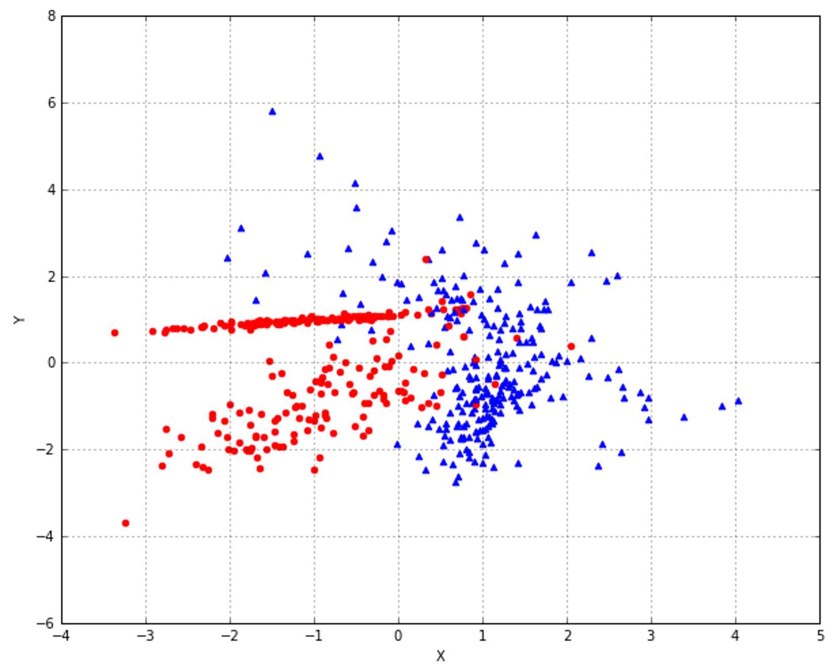 The resulting ROC curves (generated in the same way shown in the previous chapter) are shown in the following figure:得到的ROC曲线(与前一章相同方法生成)如下图所示:
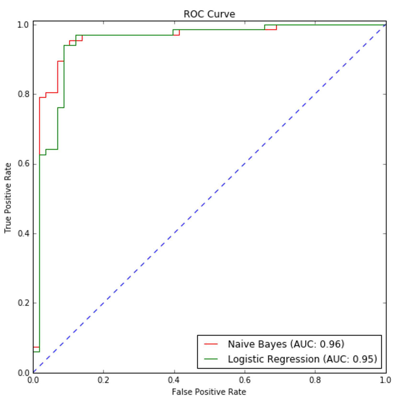 Naive Bayes' performance is slightly better than logistic regression; however, the two classifiers have similar accuracy and Area Under the Curve (AUC). It's interesting to compare the performances of Gaussian and multinomial naive Bayes with the MNIST digit dataset. Each sample (belonging to 10 classes) is an 8 x 8 image encoded as an unsigned integer (0-255); therefore, even if each feature doesn't represent an actual count, it can be considered as a sort of magnitude or frequency:朴素贝叶斯的性能略优于logistic回归;然而,这两种分类器的精度和曲线下面积(AUC)相似。比较高斯和多项式朴素贝叶斯与MNIST数字数据集的性能是很有趣的。每个样本(属于10个类)是一个8×8的图像,编码为无符号整数(0-255);因此,即使每个特征不代表一个实际的计数,它也可以被认为是一种大小或频率:
Multinomial naive Bayes performs better than the Gaussian variant and the result is not really surprising. In fact, each sample can be thought of as a feature vector derived from a dictionary of 64 symbols. The value can be the count of each occurrence, so a multinomial distribution can better fit the data, while a Gaussian is slightly more limited by its mean and variance.多项式朴素贝叶斯的性能优于高斯变种,其结果并不令人惊讶。事实上,每个样本都可以看作是从64个符号字典中派生出来的特征向量。该值可以是每次出现的次数,因此多项式分布更适合于数据,而高斯分布受均值和方差的限制略大。
特征变量由属于0-255的整数组成,高斯分布需要在均值附近更集中且值无界,显然特征变量更符合多项式分布。
datetime: 2018/11/22 21:57
6.4 References参考文献
6.5 Summary总结
7 Support Vector Machines支持向量机(SVM)
7.1 Linear support vector machines线性支持向量机(线性SVM)
Let's consider a dataset of feature vectors we want to classify:让我们考虑一个要分类的特征向量的数据集:

$$\mathbf{X}=\{\vec{x}_1,\vec{x}_2,\ldots,\vec{x}_n\} \quad where \ \vec{x}_i \in \mathbb{R}^m$$
For simplicity, we assume it as a binary classification (in all the other cases, it's possible to use automatically the one-versus-all strategy) and we set our class labels as -1 and 1:为了简单起见,我们假设它是一个二分类问题(在所有其他情况下,可以自动使用one-vs-all策略),并将类标签设置为-1和1:

$$\vec{y}=\{y_1,y_2,\ldots,y_n\} \quad where \ y_i \in \{-1,1\}$$
Our goal is to find the best separating hyperplane, for which the equation is:我们的目标是找到最佳的分离超平面,它的方程是:

$$\vec{w}^T\vec{x}+b=0 \quad where \ \vec{w}=\begin{pmatrix} w_1 \\ w_2 \\ \vdots \\ w_m \end{pmatrix} \ and \ \vec{x}=\begin{pmatrix} x_1 \\ x_2 \\ \vdots \\ x_m \end{pmatrix}$$
In the following figure, there's a bidimensional representation of such a hyperplane:在下面的图中,有这样一个超平面的二维表示:
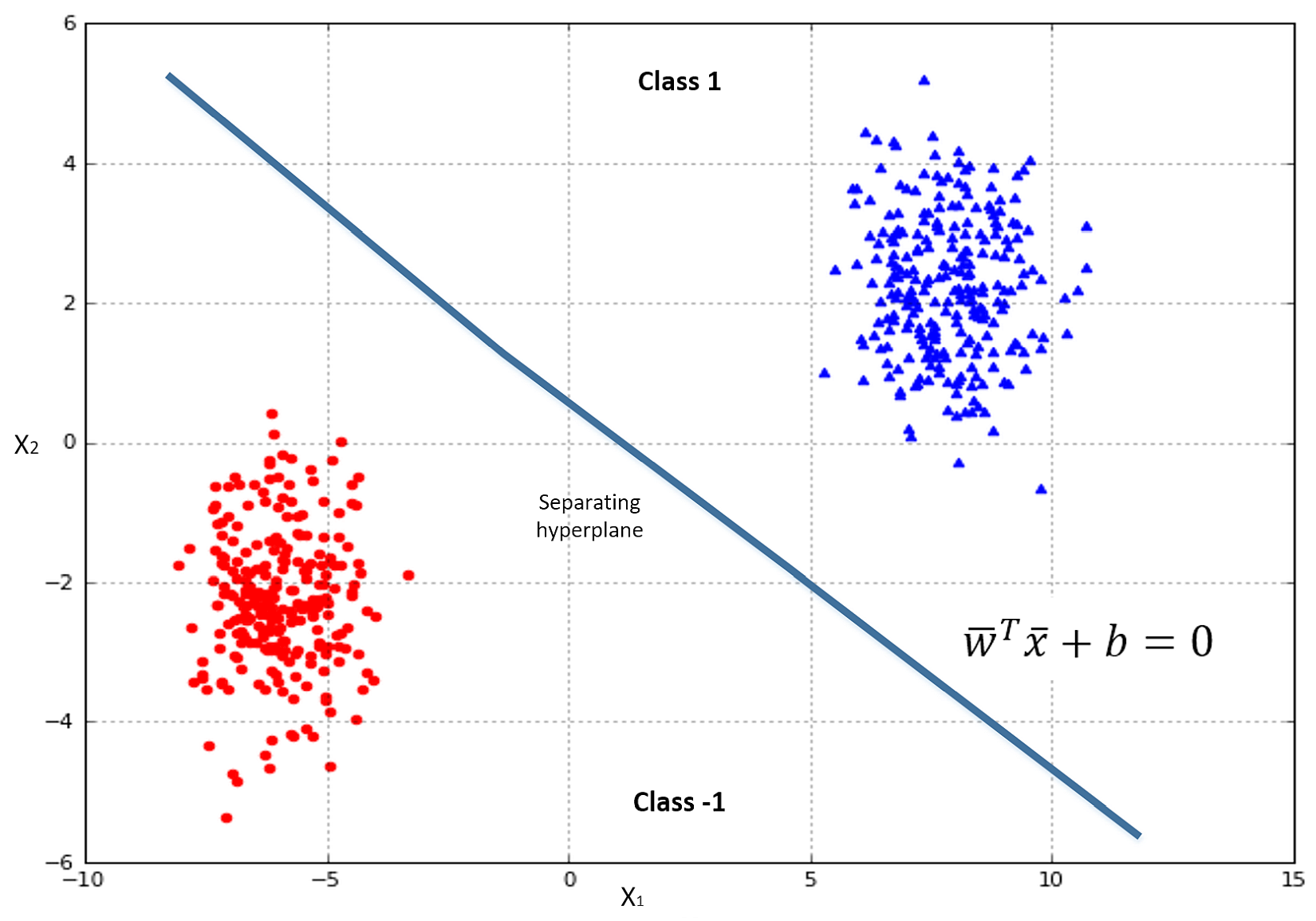 In this way, our classifier can be written as:这样,我们的分类器可以写成:

$$\hat{y}=f(\vec{x})=sgn(\vec{w}^T\vec{x}+b)$$
In a realistic scenario, the two classes are normally separated by a margin with two boundaries where a few elements lie. Those elements are called support vectors. For a more generic mathematical expression, it's preferable to renormalize our dataset so that the support vectors will lie on two hyperplanes with equations:在实际场景中,这两个类通常由两个边界分隔,边界上有一些元素。边界的元素叫做支持向量。对于更一般的数学表达式,最好将数据集重新规范化,以便支持向量位于如下超平面方程上:
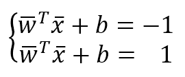
$$\left\{ \begin{aligned} \vec{w}^T\vec{x}+b & = -1 \\ \vec{w}^T\vec{x}+b & = +1 \end{aligned} \right.$$
In the following figure, there's an example with two support vectors. The dashed line is the original separating hyperplane:在下面的图中,有一个包含两个支持向量的示例。虚线是原始的分离超平面:
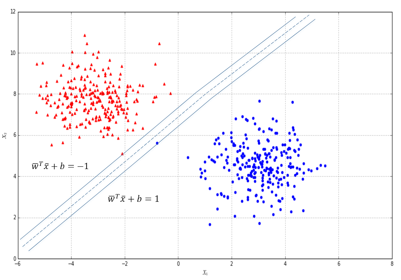 Our goal is to maximize the distance between these two boundary hyperplanes so as to reduce the probability of misclassification (which is higher when the distance is short, and there aren't two well-defined blobs as in the previous figure).我们的目标是将这两个边界超平面之间的距离最大化,从而降低错误分类的概率(当距离较短时,错误分类的概率会更高,而且不像前面的图中那样有两个定义良好的块)。
Considering that the boundaries are parallel, the distance between them is defined by the length of the segment perpendicular to both and connecting two points:考虑到边界是平行的,它们之间的距离由垂直于两条边界并连接两垂点的线段的长度来定义:
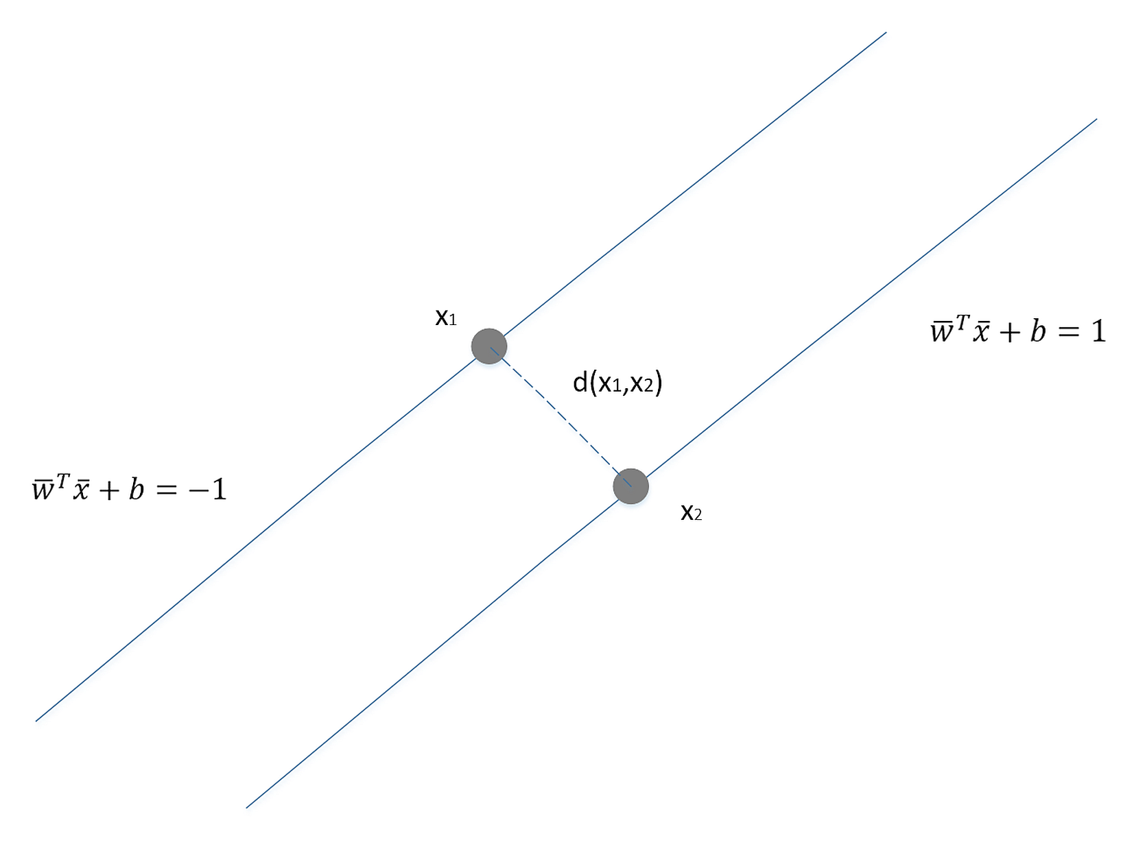 Considering the points as vectors, therefore, we have:把这些点看作向量,因此,我们有:

$$\vec{x}_2-\vec{x}_1=t\vec{w}$$
Now, considering the boundary hyperplane equations, we get:现在,考虑边界超平面方程,我们得到:

$$\vec{w}^T\vec{x}_2+b=\vec{w}^T(\vec{x}_1+t\vec{w})+b=(\vec{w}^T\vec{x}_1+b)+t\|\vec{w}\|_2^2=-1+t\|\vec{w}\|_2^2=1$$
The first term of the last part is equal to -1, so we solve for $t$:最后一部分的第一项等于-1,所以我们解出$t$:
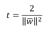
$$t=\frac{2}{\|\vec{w}\|_2^2}$$
The distance between $\vec{x}_1$ and $\vec{x}_1$ is the length of the segment $t$; hence we get: $\vec{x}_1$和$\vec{x}_1$之间的距离是线段$t$的长度;因此我们得到:

$$d(\vec{x}_1 , \vec{x}_2)=t\|\vec{w}\|_2=\frac{2}{\|\vec{w}\|_2}$$
因为线段$x_1$、$x_2$的距离为$$\|\vec{x}_2 - \vec{x}_1\|_2=\|t \vec{w}\|_2=t \|\vec{w}\|_2$$
Now, considering all points of our dataset, we can impose the following constraint:现在,考虑到数据集的所有点,我们可以施加以下约束:

$$y_i(\vec{w}^T\vec{x}_i+b) \ge 1 \quad \forall \ (\vec{x}_i,y_i)$$
This is guaranteed by using -1, 1 as class labels and boundary margins. The equality is true only for the support vectors, while for all the other points it will greater than 1. It's important to consider that the model doesn't take into account vectors beyond this margin. In many cases, this can yield a very robust model, but in many datasets this can also be a strong limitation. In the next paragraph, we're going to use a trick to avoid this rigidness while keeping the same optimization technique.这可以通过使用-1,1作为类标签和边界来保证。只有支持向量等号成立,而对于其他所有点它都大于1。很重要的一点是,模型没有考虑超出这个边界的向量。在许多情况下,这可以产生一个非常健壮的模型,但在许多数据集中,这也可能是一个很大的限制。在下一段中,我们将使用一种技巧来避免这种刚性,同时保持相同的优化技术。
At this point, we can define the function to minimize in order to train a support vector machine:在这一点上,为训练支持向量机我们可以定义函数以最小化:
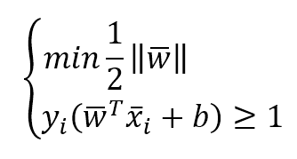
$$\left\{ \begin{aligned} & \min_{\vec{w},b}^{}{\frac{1}{2}\|\vec{w}\|_2^2} \\
& y_i(\vec{w}^T\vec{x}_i+b) \ge 1 \end{aligned} \right.$$
This can be further simplified (by removing the square root from the norm) in the following quadratic programming problem:这可以在下面的二次规划问题中进一步简化(通过从范数中去掉平方根):
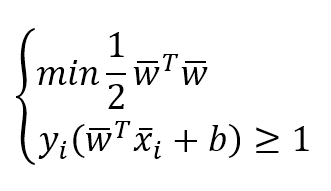
$$\left\{ \begin{aligned} & \min_{\vec{w},b}^{}{\frac{1}{2}\vec{w}^T\vec{w}} \\
& y_i(\vec{w}^T\vec{x}_i+b) \ge 1 \end{aligned} \right.$$
7.2 scikit-learn implementation scikit-learn实现
In order to allow the model to have a more flexible separating hyperplane, all scikit-learn implementations are based on a simple variant that includes so-called slack variables in the function to minimize:为了让模型具有更灵活的分离超平面,所有scikit-learn实现都基于一个简单的变体,该变体在函数中包含所谓的松弛变量以最小化:
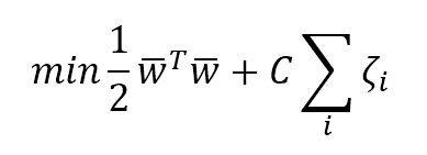
$$\min_{\vec{w},b,\zeta_i}^{}{\frac{1}{2}\vec{w}^T\vec{w}+C\sum_{i=1}^{n}{\zeta_i}}$$
In this case, the constraints become:在这种情况下,约束变成:

$$y_i(\vec{w}^T\vec{x}_i+b) \ge 1 - \zeta_i$$
松弛变量是除$\vec{w}$和$b$以外的可学习参数,对于n个样本有n个松弛参数,详见sklearn文档,我也专有一博文笔记支持向量机svm之数学原理
The introduction of the slack variables allows us to create a flexible margin so that some vectors belonging to a class can also be found in the opposite part of the hyperspace and can be included in the model training. The strength of this flexibility can be set using the parameter $C$. Small values (close to zero) bring about very hard margins, while values greater than or equal to 1 allow more and more flexibility (also increasing the misclassification rate). The right choice of $C$ is not immediate, but the best value can be found automatically by using a grid search as seen in the previous chapters.松弛变量的引入使我们能够创建一个灵活的边界,这样属于一个类的一些向量也可以在超空间的相反部分找到,并可以包含在模型训练中。可以使用参数$C$设置这种灵活性的强度。较小的值(接近于零)会带来非常硬的边界,而大于或等于1的值允许越来越多的灵活性(也会增加错误分类率)。$C$的正确选择不是立即就能得到的,但是可以通过使用网格搜索自动找到最佳值,如前几章所述。
7.2.1 Linear classification线性分类器
In the following figure, there's a plot of our dataset. Notice that some points overlap the two main blobs. For this reason, a positive C value is needed to allow the model to capture a more complex dynamic.在下面的图中,有一个数据集的图。请注意,有些点与两个主块重叠。因此,需要一个正的C值,以便模型捕获更复杂的动态。
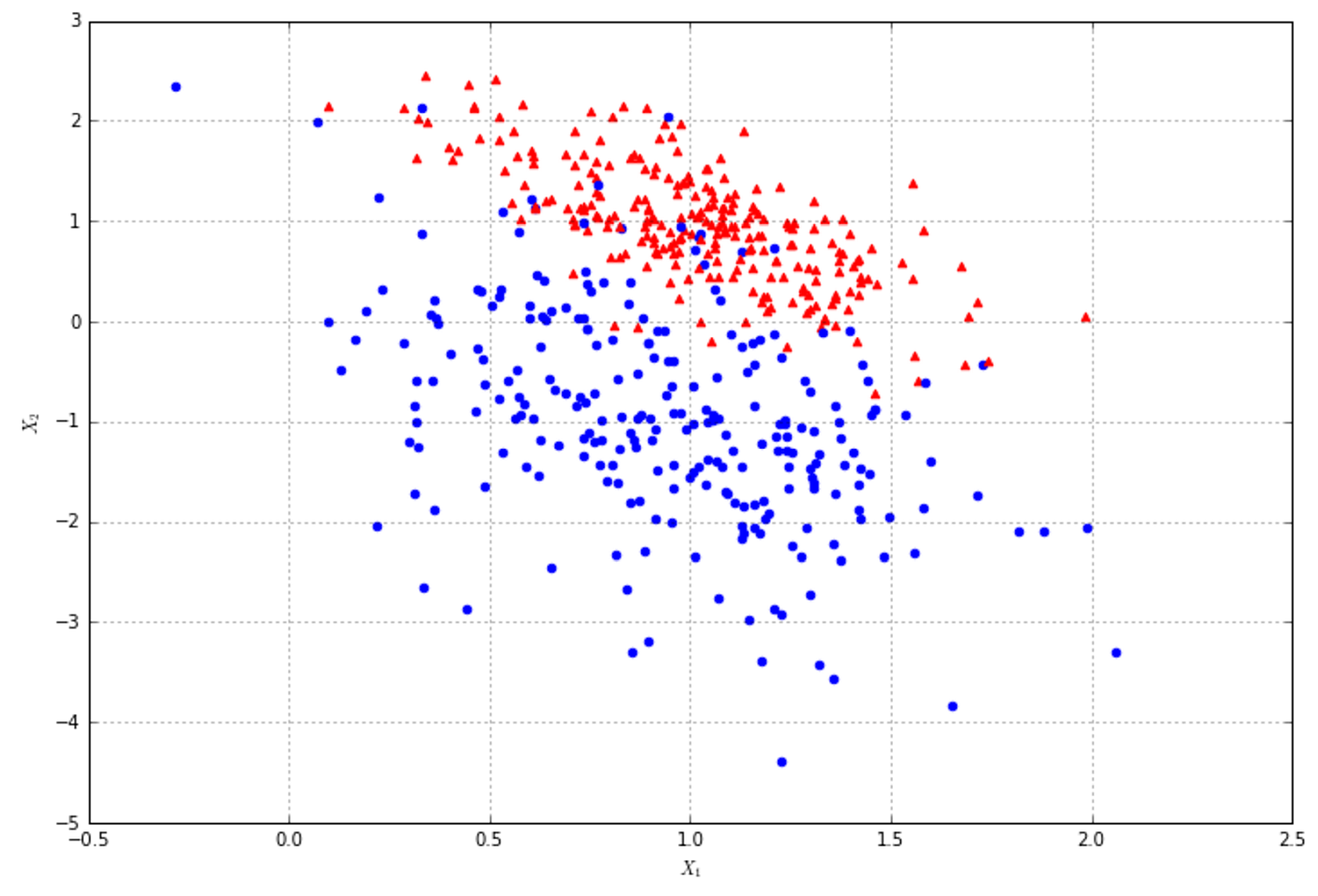 The
The kernel parameter must be set to 'linear' in this example. In the next section, we're going to discuss how it works and how it can improve the SVM's performance dramatically in non-linear scenarios. As expected, the accuracy is comparable to a logistic regression, as this model tries to find an optimal linear separator. After training a model, it's possible to get an array of support vectors, through the instance variable called support_vectors_. A plot of them, for our example, is shown in the following figure:在本例中,kernel参数必须设置为'linear'。在下一节中,我们将讨论它是如何工作的,以及如何在非线性场景中显著提高SVM的性能。正如预期的那样,由于该模型试图找到一个最优的线性分隔符,因此其准确性可与逻辑回归相媲美。在对模型进行训练之后,可以通过名为support_vectors_的实例变量获得支持向量数组。这个例子的支持向量作图如下:
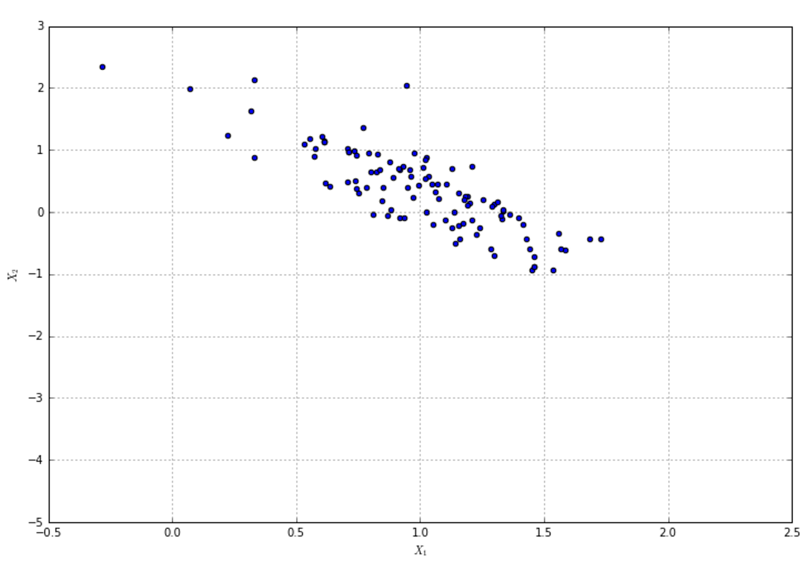
7.2.2 Kernel-based classification基于核的分类器
When working with non-linear problems, it's useful to transform the original vectors by projecting them into a higher dimensional space where they can be linearly separated. We saw a similar approach when we discussed polynomial regression. SVMs also adopt the same approach, even if there's now a complexity problem that we need to overcome. Our mathematical formulation becomes:在处理非线性问题时,将原始向量投影到高维空间中进行线性分离是很有用的。当我们讨论多项式回归时,我们看到了类似的方法。支持向量机也采用相同的方法,即使现在有一个我们需要克服的复杂问题。我们的数学公式变成:
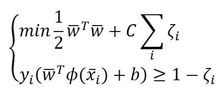
$$\left\{ \begin{aligned} & \min_{\vec{w},b}^{}{\frac{1}{2}\vec{w}^T\vec{w}+C\sum_{i=1}^{n}{\zeta_i}} \\
& y_i(\vec{w}^T\phi(\vec{x}_i)+b) \ge 1-\zeta_i \end{aligned} \right.$$
Every feature vector is now filtered by a non-linear function that can completely reshape the scenario. However, the introduction of such a function increased the computational complexity in a way that could apparently discourage this approach. To understand what has happened, it's necessary to express the quadratic problem using Lagrange multipliers. The entire procedure is beyond the scope of this book (in Nocedal J., Wright S. J., Numerical Optimization, Springer, you can find a complete and formal description of quadratic programming problems); however, the final formulation is:现在,每个特征向量都被一个非线性函数过滤,这个函数可以完全重塑场景。然而,这种函数的引入增加了计算复杂度,这显然会阻碍这种方法。为了理解发生了什么,有必要用拉格朗日乘子表示二次问题。整个过程超出本书视角,最终方程是:
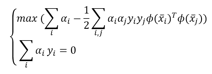
$$\left\{ \begin{aligned} & \max_{\vec{w},b}^{}{\left(\sum_{i=1}^{n}{\alpha}-\frac{1}{2}\sum_{i,j}^{n,n}{\alpha_i \alpha_j y_i y_j \phi(\vec{x}_i^T) \phi(\vec{x}_j)}\right)} \\
& \sum_{i=1}^{n}{\alpha_i y_i} = 0 \end{aligned} \right.$$
Therefore it's necessary to compute the following for every couple of vectors:因此,有必要对每一对向量计算如下:

$$\phi(\vec{x}_i^T) \phi(\vec{x}_j)$$
And this procedure can be a bottleneck, unacceptable for large problems. However, it's now that the so-called kernel trick takes place. There are particular functions (called kernels) that have the following property:这个过程可能是一个瓶颈,对于大问题来说是不可接受的。然而,现在出现了所谓的内核技巧。有一些特定的函数(称为内核)具有以下属性:

$$K(\vec{x}_i,\vec{x}_j)=\phi(\vec{x}_i^T) \phi(\vec{x}_j)$$
In other words, the value of the kernel for two feature vectors is the product of the two projected vectors. With this trick, the computational complexity remains almost the same, but we can benefit from the power of non-linear projections even in a very large number of dimensions.也就是说,两个特征向量的核的值是这两个投影向量的乘积。有了这个技巧,计算复杂度几乎保持不变,但是我们可以从非线性投影中获益,即使是在非常大的维度上。
Excluding the linear kernel, which is a simple product, scikit-learn supports three different kernels that can solve many real-life problems.排除线性内核(这是一个简单的产品),scikit-learn支持三个不同的内核,可以解决许多实际问题。
7.2.2.1 Radial Basis Function径向基函数
The RBF kernel is the default value for SVC and is based on the function:RBF内核是SVC的默认值,它是基于函数:

$$K(\vec{x}_i,\vec{x}_j)=e^{-\gamma{|\vec{x}_i-\vec{x}_i|}^2}$$
The gamma parameter determines the amplitude of the function, which is not influenced by the direction but only by the distance.伽马参数决定了函数的振幅,它不受方向的影响,只受距离的影响。
7.2.2.2 Polynomial kernel多项式核
The polynomial kernel is based on the function:多项式核是基于函数:

$$K(\vec{x}_i,\vec{x}_j)={\left(\gamma \vec{x}_i^T \cdot \vec{x}_j + r\right)}^c$$
The exponent c is specified through the parameter degree, while the constant term r is called coef0. This function can easily expand the dimensionality with a large number of support variables and overcome very non-linear problems; however, the requirements in terms of resources are normally higher. Considering that a non-linear function can often be approximated quite well for a bounded area (by adopting polynomials), it's not surprising that many complex problems become easily solvable using this kernel.指数c通过参数度指定,常数项r称为coef0。该函数可以方便地用大量的支持变量扩展维数,克服非常非线性的问题;但是,资源方面的要求通常较高。考虑到一个非线性函数通常可以很好地逼近一个有界区域(通过使用多项式),使用这个核可以很容易地解决许多复杂的问题也就不足为奇了。
7.2.2.3 Sigmoid kernel Sigmoid核
The sigmoid kernel is based on this function: sigmoid内核是基于函数:

$$K(\vec{x}_i,\vec{x}_j)=\frac{1-e^{-2(\gamma \vec{x}_i^T \cdot \vec{x}_j + r)}}{1+e^{-2(\gamma \vec{x}_i^T \cdot \vec{x}_j + r)}}$$
The constant term r is specified through the parameter coef0.常数项r通过参数coef0指定。
7.2.2.4 Custom kernels 自定义核
7.2.3 Non-linear examples 非线性例子
A plot of this dataset is shown in the following figure:下图显示了该数据集的作图:
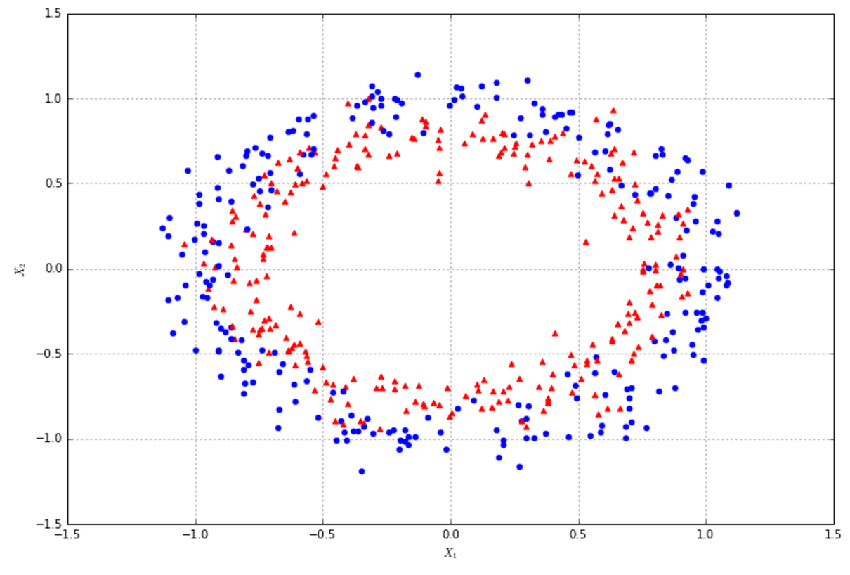 A subset of samples is shown in the following figure:下图显示了示例的一个子集:
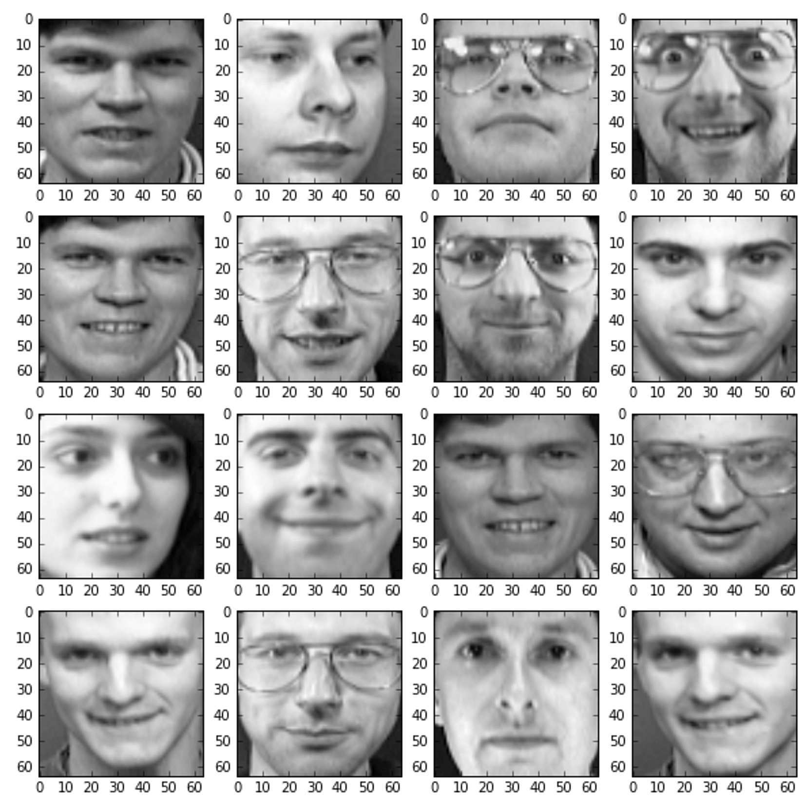
7.3 Controlled support vector machines受控制的支持向量机(受控制的SVM)
With real datasets, SVM can extract a very large number of support vectors to increase accuracy, and that can slow down the whole process. To allow finding out a trade-off between precision and number of support vectors, scikit-learn provides an implementation called NuSVC, where the parameter nu (bounded between 0—not included—and 1) can be used to control at the same time the number of support vectors (greater values will increase their number) and training errors (lower values reduce the fraction of errors). In the following figure, there's a scatter plot of our set:利用真实数据集,支持向量机可以提取大量的支持向量来提高精度,但会降低整个过程的速度。允许发现之间的权衡精度和数量的支持向量,scikit-learn提供了一个叫做NuSVC实现,参数nu(0-1之间,不包括0但包括1)可以用来同时控制支持向量的个数(更大的值将会增加他们的数量)和培训错误(更小的值减少错误)。下图是数据集的散点图:
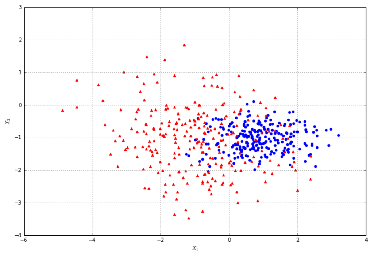
7.4 Support vector regression支持向量回归
The dataset in plotted in the following figure:数据集作图如下:
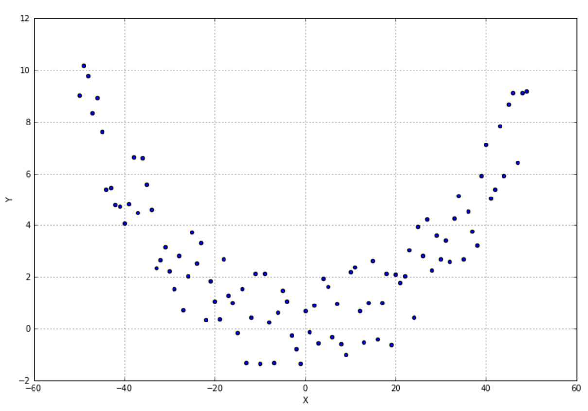
7.5 References参考文献
7.6 Summary总结
datetime: 2018/12/18/ 17:08