机器学习算法machine_learning_algorithms_2
8 Decision Trees and Ensemble Learning决策树和集成学习
8.1 Binary decision trees二分类决策树
决策树的公式基本都是错误的,请参阅我的博文笔记决策树decision_tree。
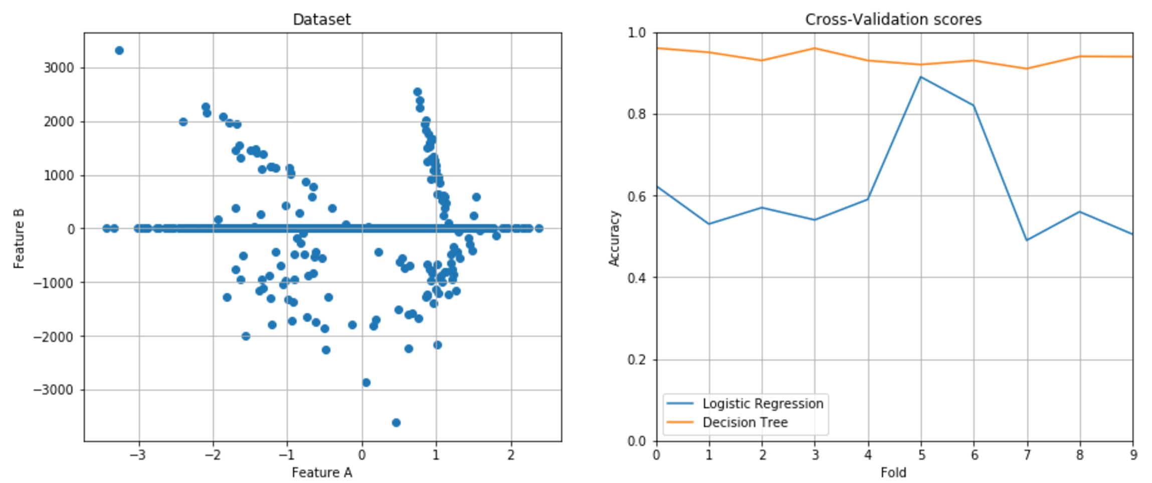
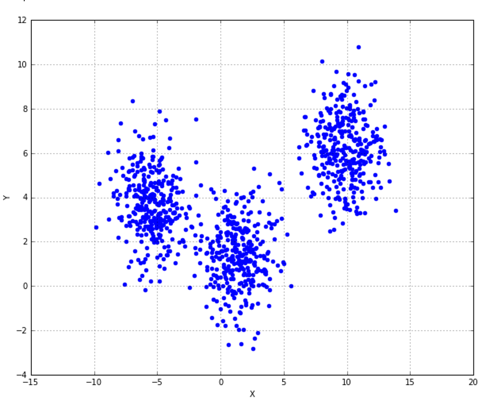
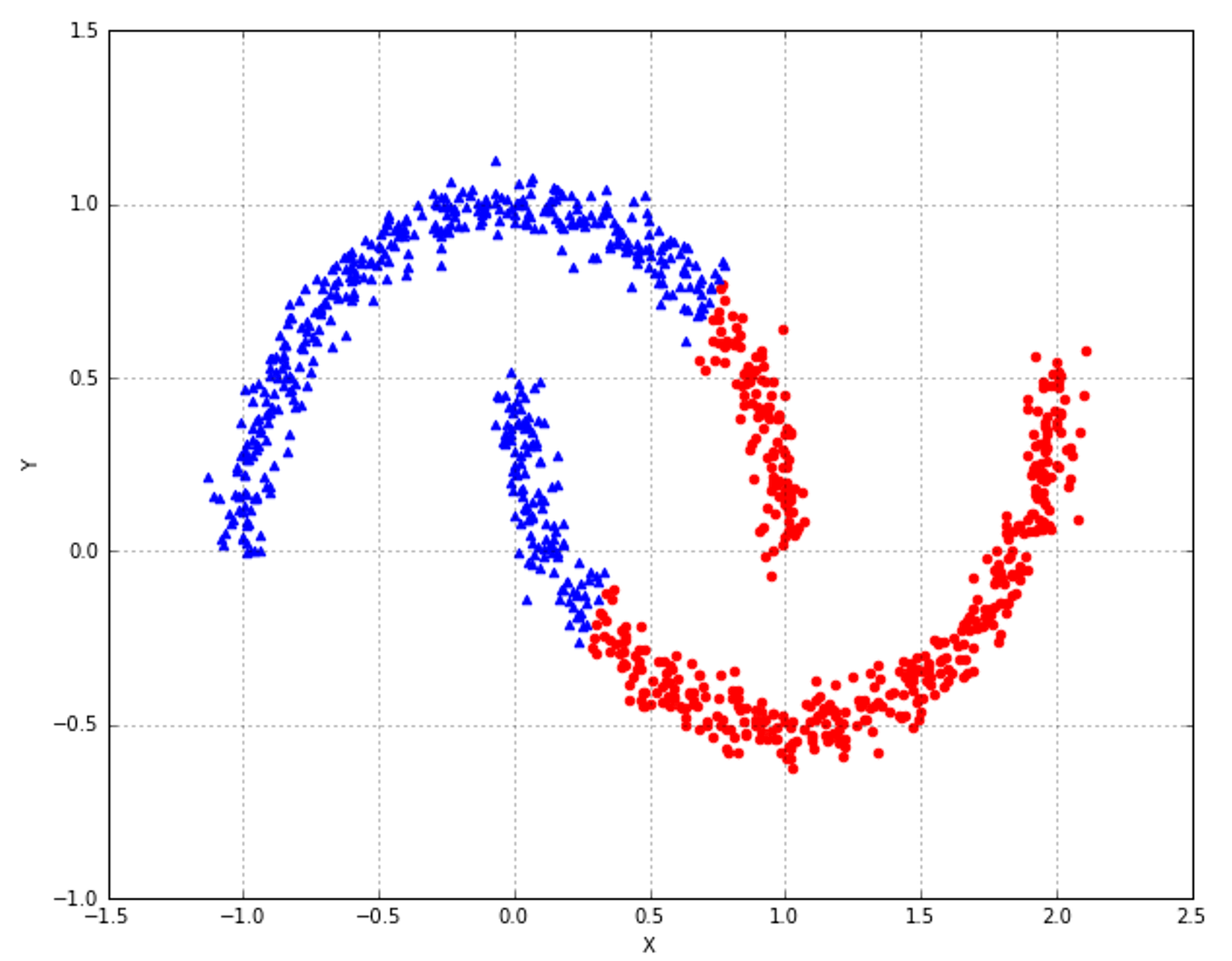
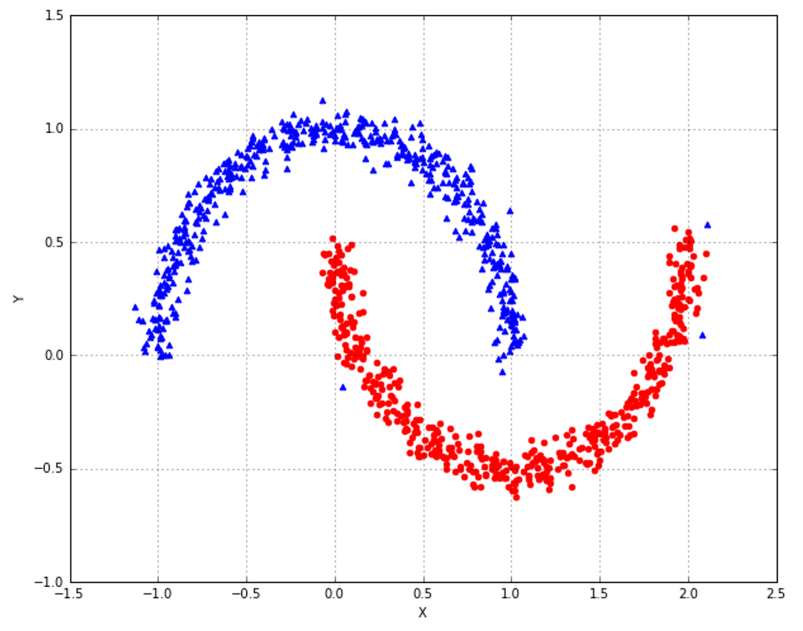
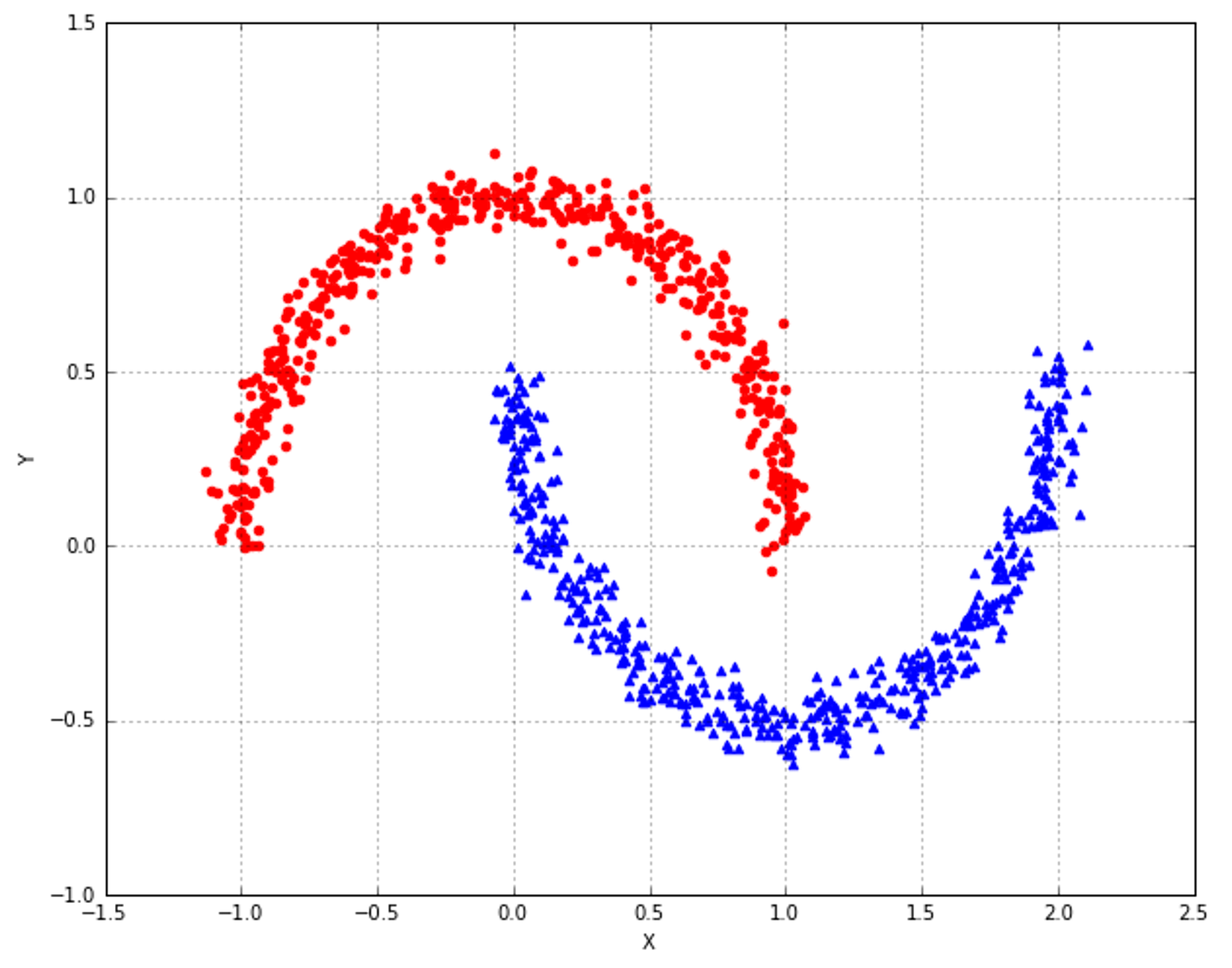
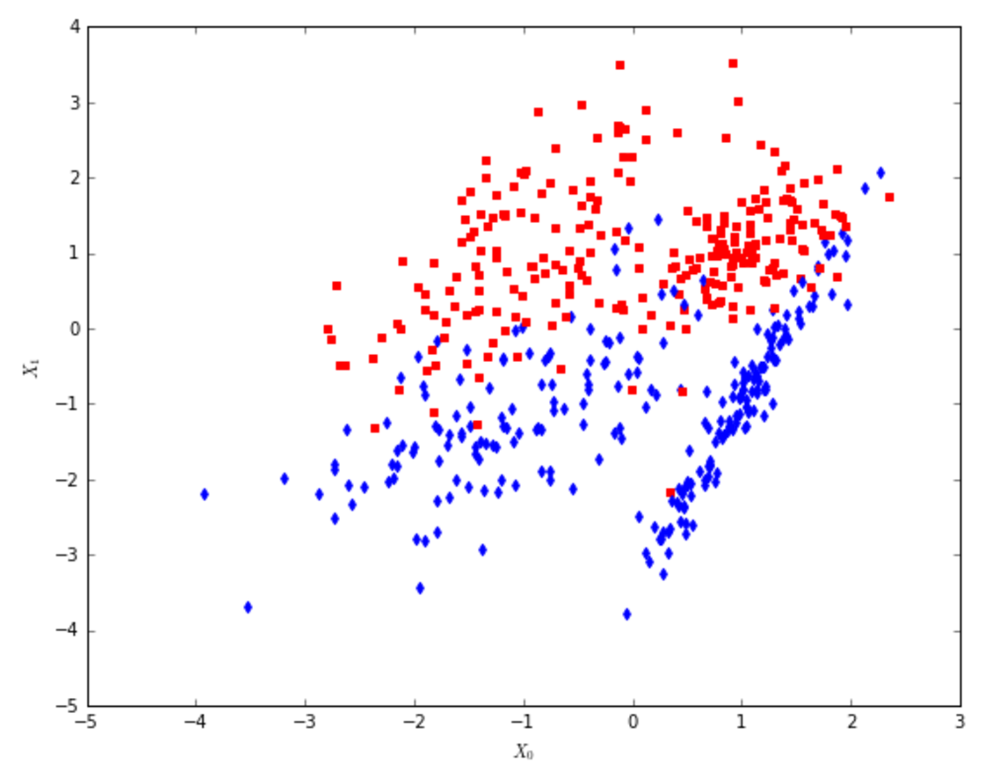
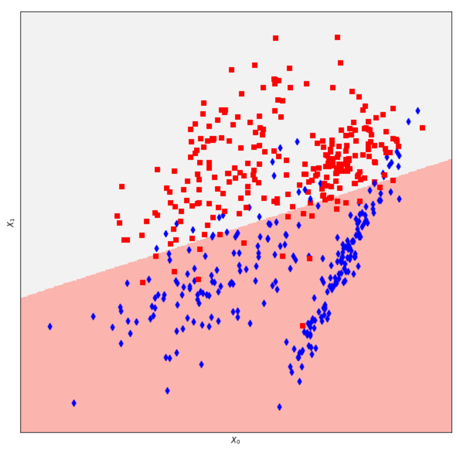
In the following figure, there are plots of an unnormalized bidimensional dataset and the cross-validation scores obtained using a logistic regression and a decision tree:下图是一个未归一化的二维数据集,以及使用逻辑回归和决策树得到的交叉验证得分:
8.1.1 Binary decisions二分类决策
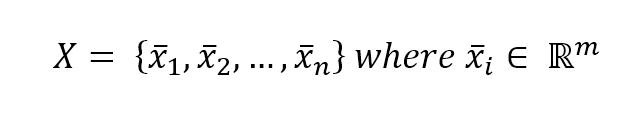
Let's consider an input dataset $\mathbf{X}$:让我们考虑一个输入数据集$\mathbf{X}$:

$$\mathbf{X}=\{\vec{x}_1, \vec{x}_2, \ldots, \vec{x}_n\} \ where \ \vec{x}_i \in \mathbb{R}^m$$
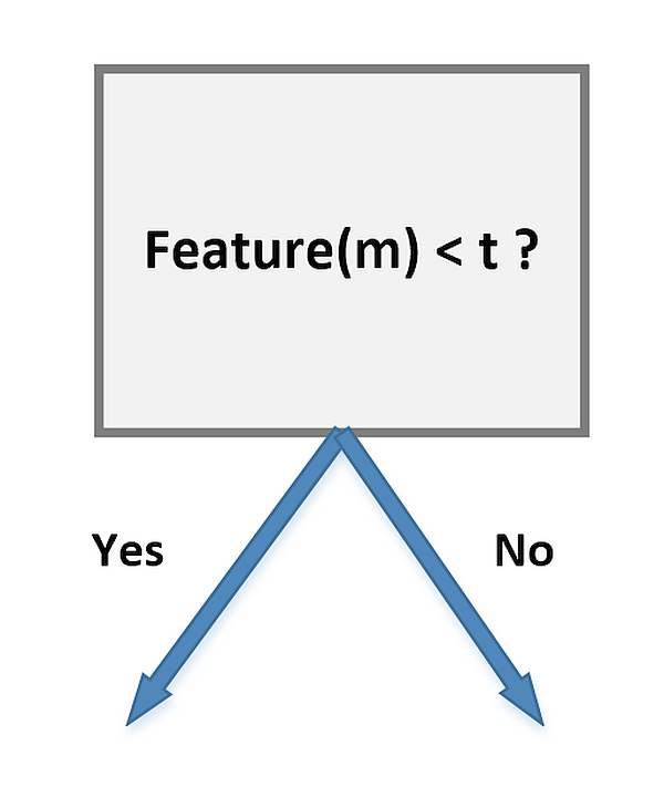
Every vector is made up of $m$ features, so each of them can be a good candidate to create a node based on the (feature, threshold) tuple:每个向量由$m$个特征组成,因此每个特征都是基于(特征、阈值)元组创建节点的良好候选:
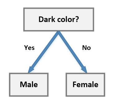
 For example, let's consider a class of students where all males have dark hair and all females have blonde hair, while both subsets have samples of different sizes. If our task is to determine the composition of the class, we can start with the following subdivision:例如,让我们考虑一个班级,所有的男生都是黑发,所有的女生都是金发,而两个子集的样本大小不同。如果我们的任务是确定类的组成,我们可以从下面的细分开始:
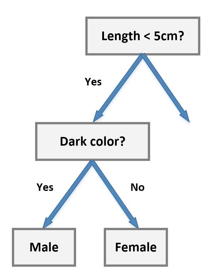 However, the block Dark color? will contain both males and females (which are the targets we want to classify). This concept is expressed using the term purity (or, more often, its opposite concept, impurity). An ideal scenario is based on nodes where the impurity is null so that all subsequent decisions will be taken only on the remaining features. In our example, we can simply start from the color block:但是,色块深色与否将包含男性和女性(这是我们要分类的目标)。这个概念是用“纯度”一词来表示的(或者,更经常地,它的相反概念是“不纯度”)。理想的场景是基于不纯度为null的节点,这样以后所有的决定都将只针对剩下的特性做出。在我们的例子中,我们可以简单地从颜色块开始:
 More formally, suppose we define the selection tuple as:更正式地说,假设我们将选择元组定义为:
$$\sigma = \langle i, t_k \rangle$$
Here, the first element is the index of the feature we want to use to split our dataset at a certain node (it will be the entire dataset only at the beginning; after each step, the number of samples decreases), while the second is the threshold that determines left and right branches. The choice of the best threshold is a fundamental element because it determines the structure of the tree and, therefore, its performance. The goal is to reduce the residual impurity in the least number of splits so as to have a very short decision path between the sample data and the classification result. 在这里,第一个元素是我们想要用来在某个节点上分割数据集的特性的索引(它只在开始时是整个数据集;在每一步之后,样本的数量会减少),而第二个元素是决定左右分支的阈值。最佳阈值的选择是一个基本元素,因为它决定了树的结构,因此也决定了树的性能。其目的是在最小分割次数内减少残余不纯度,使样本数据与分类结果之间的决策路径非常短。
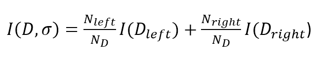
We can also define a total impurity measure by considering the two branches:我们也可以通过考虑以下两个分支来定义不纯度度量:
$$I(\mathbf{D},\sigma)=\frac{N_{left}}{N_\mathbf{D}}I(\mathbf{D}_{left})+\frac{N_{right}}{N_\mathbf{D}}I(\mathbf{D}_{right})$$
Here, $\mathbf{D}$ is the whole dataset at the selected node, $\mathbf{D}_{left}$ and $\mathbf{D}_{right}$ are the resulting subsets (by applying the selection tuple), and the $I$ are impurity measures.这里,$\mathbf{D}$是所选节点的整个数据集,$\mathbf{D}_{left}$和$\mathbf{D}_{right}$是结果子集(通过应用选择元组),$I$是不纯度度量。
8.1.2 Impurity measures不纯度测量
To define the most used impurity measures, we need to consider the total number of target classes:为了定义最常用的杂质测量,我们需要考虑目标类的总数:
$$\vec{y}=\{y_1,y_2,\ldots,y_n\} \ where \ y_i \in \{0,1,2,\ldots,P\}$$
In a certain node $j$, we can define the probability $p(i|j)$ where i is an index $i \in \{0,1,2,\ldots,n\}$ associated with each class. In other words, according to a frequentist approach, this value is the ratio between the number of samples belonging to class $i$ and the total number of samples belonging to the selected node.在某个节点$j$中,我们可以定义概率$p(i|j)$,其中i是与每行分类关联的索引$i \in \{0,1,2,\ldots,n\}$(撤这多淡,作者意思$i$是行索引)。换句话说,根据频率主义者的方法,这个值是属于第$i$类的样本数与属于所选节点的样本总数之比。
8.1.2.1 Gini impurity index基尼不纯度指数
The Gini impurity index is defined as:基尼不纯度指数定义为:
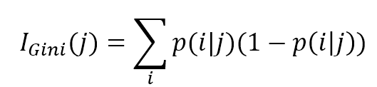
$$I_{Gini}(j)=\sum_{i}^{}{p(i|j)\left(1-p(i|j)\right)}$$
Here, the sum is always extended to all classes. This is a very common measure and it's used as a default value by scikit-learn. Given a sample, the Gini impurity measures the probability of a misclassification if a label is randomly chosen using the probability distribution of the branch. The index reaches its minimum (0.0) when all the samples of a node are classified into a single category.在这里,总和总是扩展到所有类。这是一个非常常见的度量方法,它被scikit-learn用作默认值。给定样本,如果使用分支的概率分布随机选择一个标签,则基尼不纯度测量错误分类的概率。当节点的所有样本都被归为一个类别时,指数达到最小值(0.0)。
8.1.2.2 Cross-entropy impurity index交叉不纯度指数
The cross-entropy measure is defined as:交叉熵测度定义为:
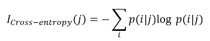
$$I_{Cross-entropy}(j)=-\sum_{i}^{}{p(i|j)\log{p(i|j)}}$$
This measure is based on information theory, and assumes null values only when samples belonging to a single class are present in a split, while it is maximum when there's a uniform distribution among classes (which is one of the worst cases in decision trees because it means that there are still many decision steps until the final classification). This index is very similar to the Gini impurity, even though, more formally, the cross-entropy allows you to select the split that minimizes the uncertainty about the classification, while the Gini impurity minimizes the probability of misclassification.这个测量是基于信息理论,假定null值只有当样本都划入一个类,而类间均匀分布时达到最大值(这是决策树最糟糕的情况,因为这意味着仍有许多决策步骤,直到最终的分类)。该指标与基尼系数非常相似,尽管更正式地说,交叉熵允许您选择能够最小化分类不确定性的分割,而基尼系数则可以最小化错误分类的概率。
In Chapter 2, Important Elements in Machine Learning, we defined the concept of mutual information $I(X; Y) = H(X) - H(X|Y)$ as the amount of information shared by both variables, thereby reducing the uncertainty about $X$ provided by the knowledge of $Y$. We can use this to define the information gain provided by a split:在第二章机器学习的重要元素中,我们定义了互信息$I(X; Y) = H(X) - H(X|Y)$作为两个变量共享的信息量,从而减少了$Y$知识提供的关于$X$的不确定性。我们可以使用它来定义分割提供的信息增益:
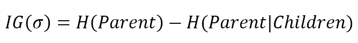
$$IG(\sigma)=H(Parent)-H(Parent|Children)$$
When growing a tree, we start by selecting the split that provides the highest information gain and proceed until one of the following conditions is verified:在生成树时,我们首先选择提供最高信息增益的分割,然后继续,直到验证以下条件之一:
- All nodes are pure 所有节点都纯净
- The information gain is null 信息增益为零
- The maximum depth has been reached 已达到最大深度
8.1.2.3 Misclassification impurity index误分类不纯度指数
The misclassification impurity is the simplest index, defined as:误分类不纯度是最简单的指标,定义为:
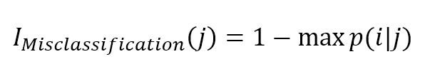
$$I_{Misclassification}(j)=1-\max{p(i|j)}$$
In terms of quality performance, this index is not the best choice because it's not particularly sensitive to different probability distributions (which can easily drive the selection to a subdivision using Gini or cross-entropy indexes).就质量性能而言,这个指数不是最佳选择,因为它对不同的概率分布不是特别敏感(使用基尼系数或交叉熵索引可以很容易地将选择驱动到细分)。
8.1.3 Feature importance特征重要度
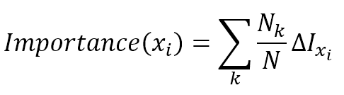
When growing a decision tree with a multidimensional dataset, it can be useful to evaluate the importance of each feature in predicting the output values. In Chapter 3, Feature Selection and Feature Engineering, we discussed some methods to reduce the dimensionality of a dataset by selecting only the most significant features. Decision trees offer a different approach based on the impurity reduction determined by every single feature. In particular, considering a feature xi, its importance can be determined as:在使用多维数据集生成决策树时,评估每个特性在预测输出值方面的重要性是很有用的。在第三章,特征选择和特征工程中,我们讨论了通过只选择最重要的特征来降低数据集维数的一些方法。决策树提供了一种不同的方法,它基于每个特征所决定的不纯度下降。特别是考虑到一个特征$\vec{x}_i$,其重要性可以确定为:
 【
数据集
【
数据集$\mathbf{D}$有$m$个特征,经多个节点$\sigma = \langle i, t_k \rangle$划分至满足迭代停止条件(对回归只能是达到预设深度),其中$\sigma_1,\sigma_2,\ldots,\sigma_k$为根据特征列$\vec{x}_i$划分,那么据特征列$\vec{x}_i$的重要性可由下式计算:
$${Importance}(\vec{x}_i)=\frac{\Delta{I(\vec{x}_i)}}{\sum_{i=1}^{m}{\Delta{I(\vec{x}_i)}}} \\
where \ \Delta{I(\vec{x}_i)}=\sum_{j=1}^{k}{\Delta{I(\sigma_j)}}=\sum_{j=1}^{k}{\left(\Delta{I(without \ \sigma_j)-I(with \ \sigma_j)}\right)}$$
】
The sum is extended to all nodes where $\vec{x}_i$ is used, and $N_k$ is the number of samples reaching the node $k$. Therefore, the importance is a weighted sum of all impurity reductions computed considering only the nodes where the feature is used to split them. If the Gini impurity index is adopted, this measure is also called Gini importance.和扩展到使用$\vec{x}_i$的所有节点,$N_k$是到达节点$k$的样本数量。因此,重要性是计算出的所有不纯度减少量的加权和,这些减少量只考虑特征用于分割它们的节点。如果采用基尼系数不纯度指数,也称为基尼系数重要度。
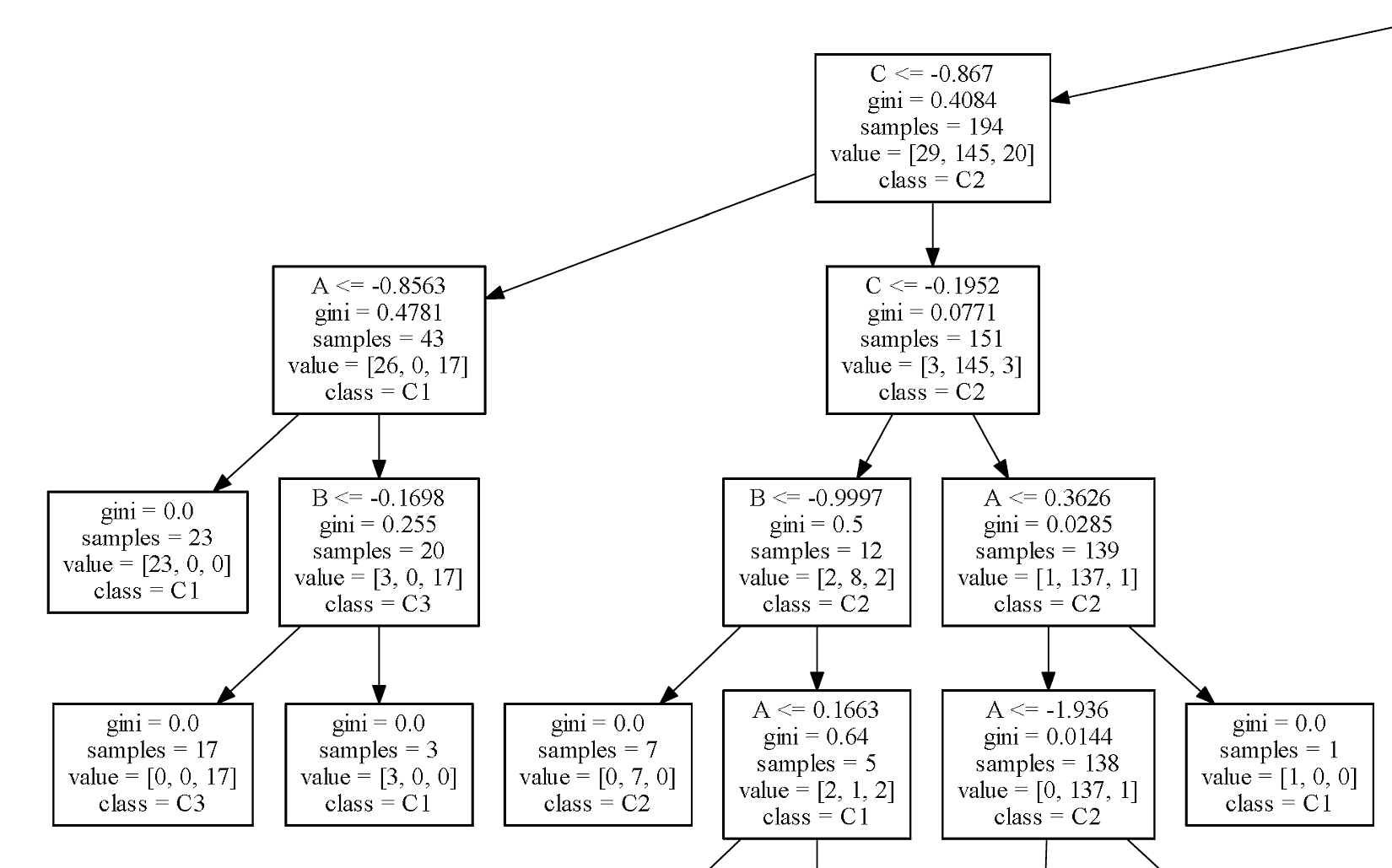
8.2 Decision tree classification with scikit-learn 采用scikit-learn的决策树分类器
The graph for our example is rather large, so in the following feature you can see only a part of a branch:我们示例的图形相当大,因此在下面的特性中只能看到分支的一部分:
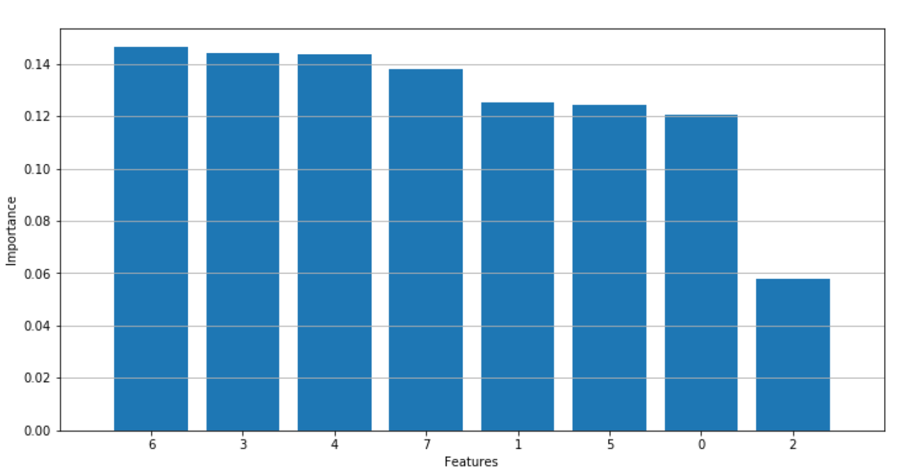
 The following figure shows a plot of the importances:下图显示了重要度的图表:
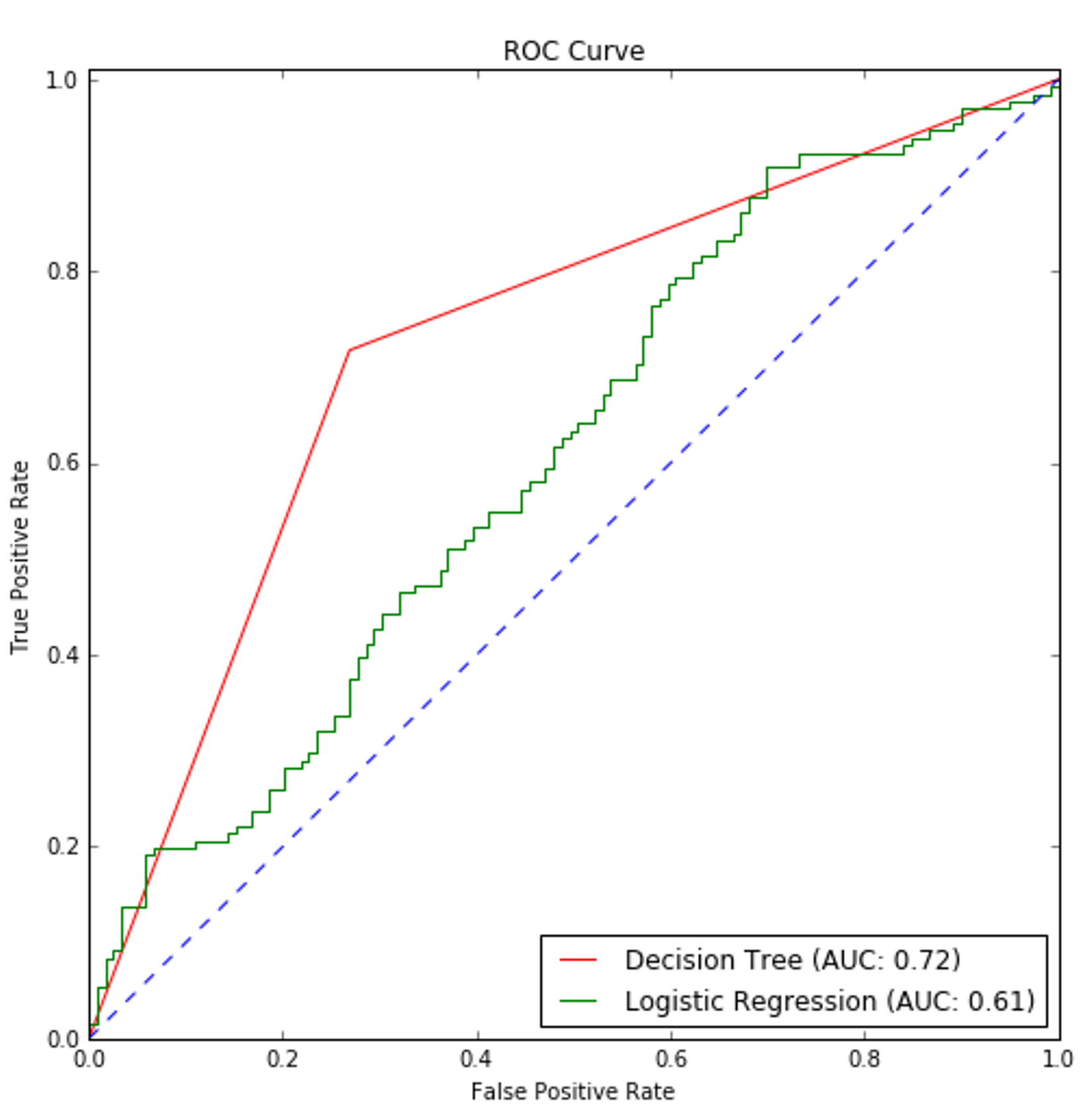
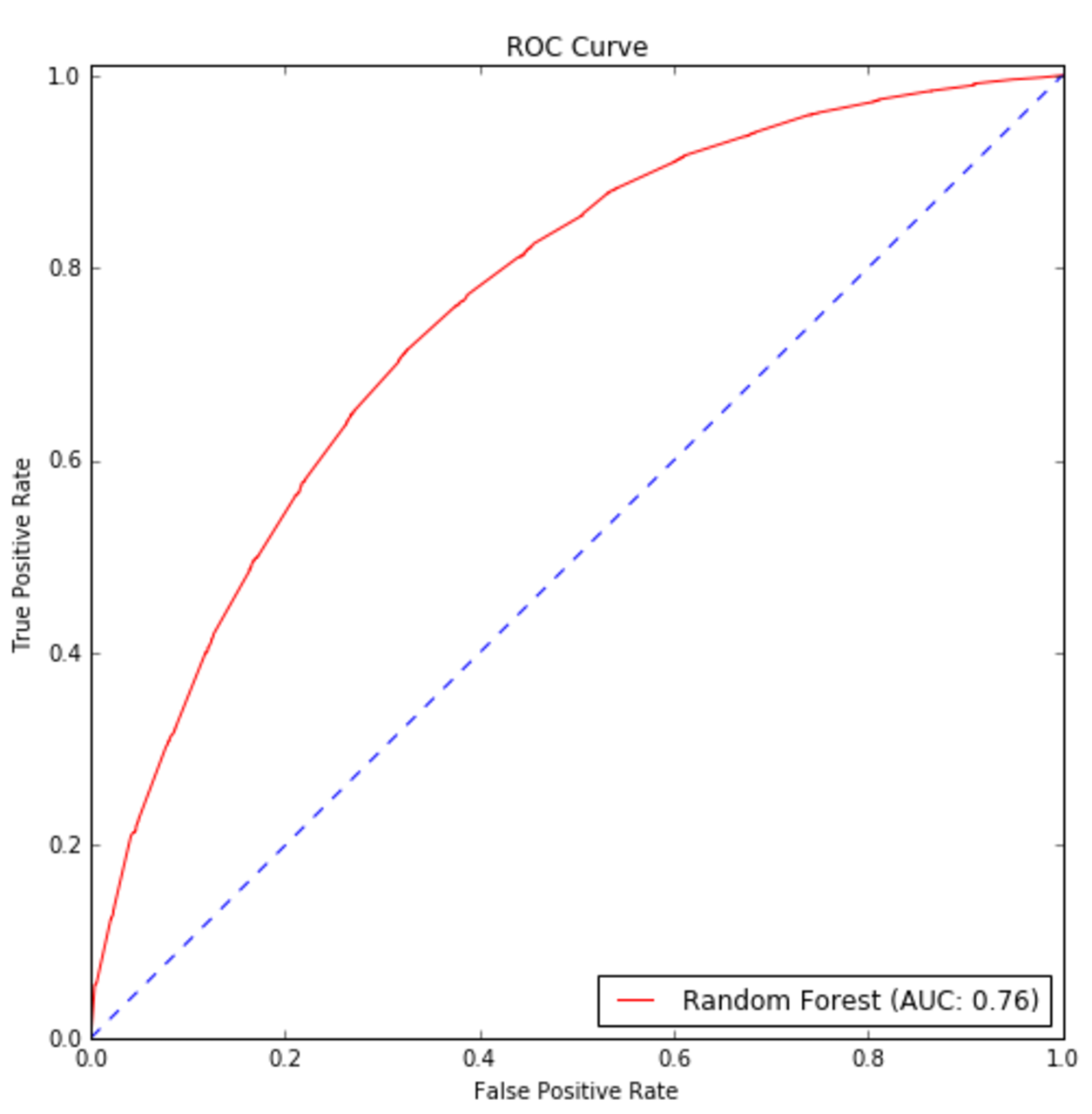
 The resulting ROC curve is shown in the following figure:得到的ROC曲线如下图所示:
8.3 Ensemble learning集成学习
Until now, we have trained models on single instances, iterating an algorithm in order to minimize a target loss function. This approach is based on so-called strong learners, or methods that are optimized to solve a specific problem by looking for the best possible solution. Another approach is based on a set of weak learners that can be trained in parallel or sequentially (with slight modifications on the parameters) and used as an ensemble based on a majority vote or the averaging of results. These methods can be classified into two main categories:到目前为止,我们已经在单个实例上训练了模型,迭代算法以最小化目标损失函数。这种方法基于所谓的“强学习者”,即通过寻找可能的最佳解决方案来优化解决特定问题。另一种方法是建立在一组弱学习者的基础上,这些弱学习者可以被并行或顺序地训练(对参数稍加修改),并作为基于多数投票或结果平均的集合使用。这些方法可以分为两大类:
- Bagged (or Bootstrap) trees: In this case, the ensemble is built completely. The training process is based on a random selection of the splits and the predictions are based on a majority vote. Random forests are an example of bagged tree ensembles.打包树(或者自助树):在这种情况下,集成是完全构建的。训练过程是基于对分裂的随机选择,预测是基于多数投票。随机森林是打包树集成学习的一个例子。
- Boosted trees: The ensemble is built sequentially, focusing on the samples that have been previously misclassified. Examples of boosted trees are AdaBoost and gradient tree boosting.增强树:该集成是按顺序构建的,关注之前被错误分类的样本。增强树的例子有AdaBoost和gradient tree boosting。
以上是书作者的原话,由于名字不好翻译,我查阅了sklearn文档,文档是这么说的:
Two families of ensemble methods are usually distinguished: * In averaging methods, the driving principle is to build several estimators independently and then to average their predictions. On average, the combined estimator is usually better than any of the single base estimator because its variance is reduced. Examples: Bagging methods, Forests of randomized trees, …在平均方法中,驱动原理是独立构建多个估计量,然后对它们的预测进行平均。通过平均,组合估计量通常优于任何单个基本估计量,因为它的方差减小了。例子:Bagging方法和随机森林等。 * By contrast, in boosting methods, base estimators are built sequentially and one tries to reduce the bias of the combined estimator. The motivation is to combine several weak models to produce a powerful ensemble. Examples: AdaBoost, Gradient Tree Boosting, …相反,在增强方法中,基本估计量是按顺序建立的,并试图减少组合估计量的偏差。其动机是将几个弱模型组合成一个强大的集成。例子:AdaBoost和Gradient Tree Boosting等。
8.3.1 Random forests随机森林
A random forest is a set of decision trees built on random samples with a different policy for splitting a node: Instead of looking for the best choice, in such a model, a random subset of features (for each tree) is used, trying to find the threshold that best separates the data. As a result, there will be many trees trained in a weaker way and each of them will produce a different prediction.随机森林是建立在随机样本并有不同的分裂一个节点策略一组决策树的合集:不寻找最好的选择,每个树模型寻找并使用一个随机特性的子集(每棵树),树的合集也就是随机森林模型试图找到最佳的阈值分隔数据。因此,将有许多树,每个树训练一个弱分类器并产生不同的预测。
There are two ways to interpret these results; the more common approach is based on a majority vote (the most voted class will be considered correct). However, scikit-learn implements an algorithm based on averaging the results, which yields very accurate predictions. Even if they are theoretically different, the probabilistic average of a trained random forest cannot be very different from the majority of predictions (otherwise, there should be different stable points); therefore the two methods often drive to comparable results.有两种方法来解释这些结果;更常见的方法是基于多数投票(投票最多的类将被认为是正确的)。然而,scikit-learn实现了一种基于平均结果的算法,它可以产生非常准确的预测。即使它们在理论上是不同的,经过训练的随机森林的概率平均值也不能与大多数预测有很大的不同(否则,就应该有不同的稳定点。译者注:这个稳定点按我理解就是n_estimators,也就是树的数目。);因此,这两种方法往往能产生相当的结果。
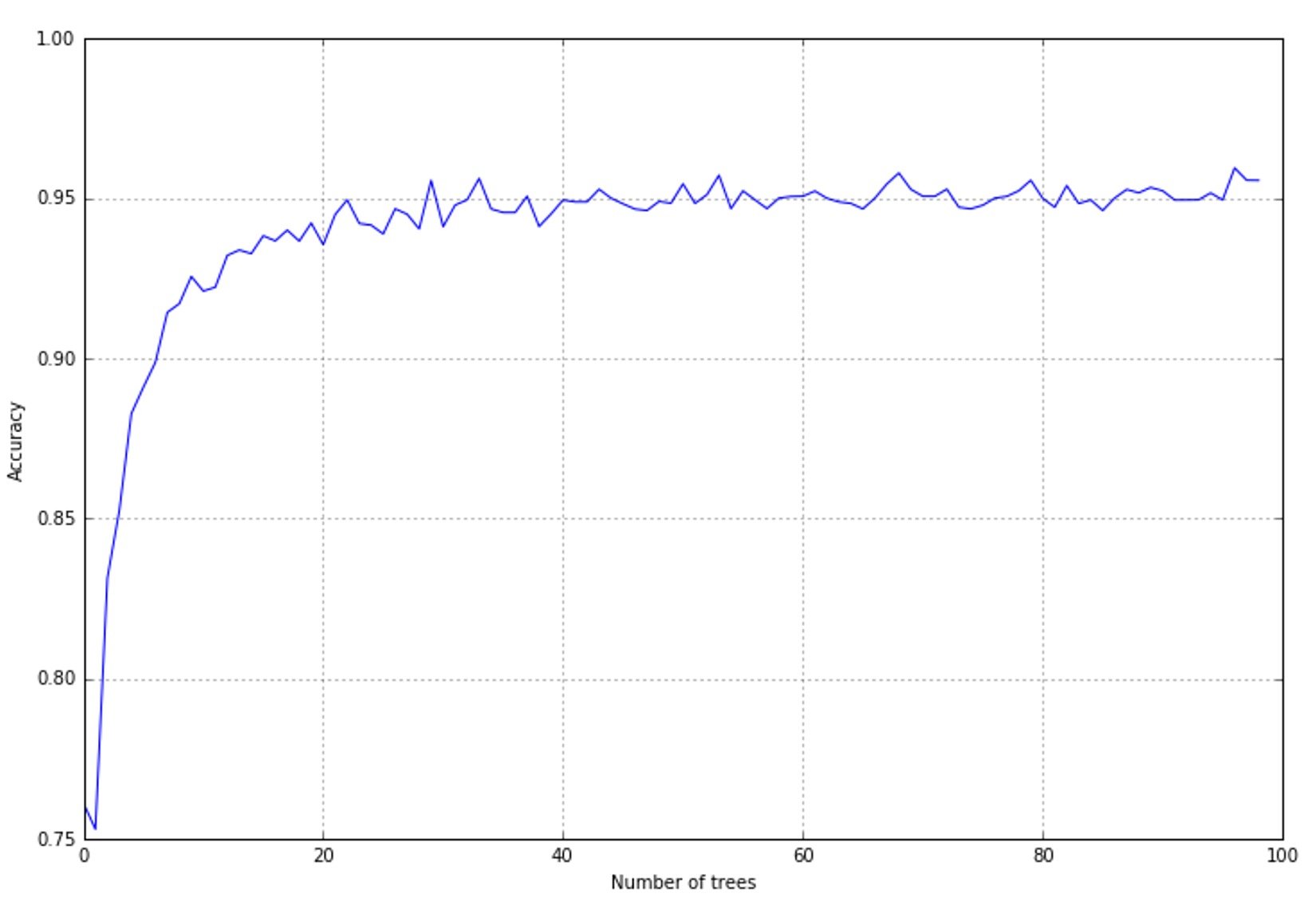
The resulting plot is shown in the following figure:结果图如下图所示:
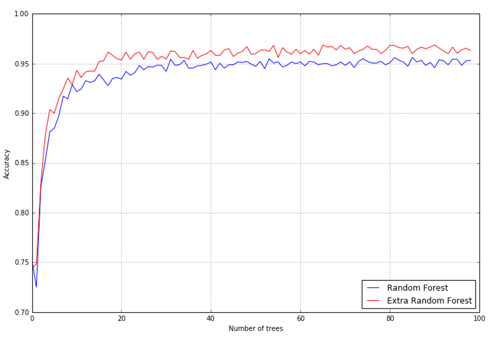
The results (with the same number of trees) in terms of accuracy are slightly better, as shown in the following figure:在精度方面,(extra-trees比 random forest)结果要好一点,如下图所示:
但是为什么两者结果会不同,以上也没有说清楚两者的差别,现在暂时没搞清楚。我想先放下,待学完整章有了更清晰的认识或许能弄明白,这里的细节绝不可放过,很重要!!!!!!!!!!!!!!!!!!!!还有lightgb、catgb、xgboost应该也是与这些相关大的,也不可放过!!!!!!!!!!
对比ExtraTreesClassifier和RandomForestClassifier参数相同,唯一不同是ExtraTreesClassifier默认bootstrap=False而RandomForestClassifier默认bootstrap=True。查阅sklearn文档有如下话语:n extremely randomized trees (see ExtraTreesClassifier and ExtraTreesRegressor classes), randomness goes one step further in the way splits are computed. As in random forests, a random subset of candidate features is used, but instead of looking for the most discriminative thresholds, thresholds are drawn at random for each candidate feature and the best of these randomly-generated thresholds is picked as the splitting rule. This usually allows to reduce the variance of the model a bit more, at the expense of a slightly greater increase in bias:
8.3.1.1 Feature importance in random forests随机森林中的特征重要性
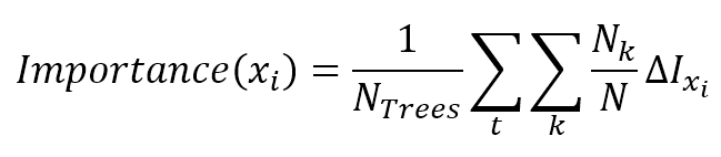
$${Importance}(\vec{x}_i)=\frac{}{N_{Trees}}\sum_{t}^{}{\sum_{k}^{}{\frac{N_k}{N}\triangle I_{\vec{x}_i}}}$$
The importance of the first 50 features according to a random forest with 20 trees is plotted in the following figure:根据一个20棵树的随机森林,前50个特征的重要性如下图所示:
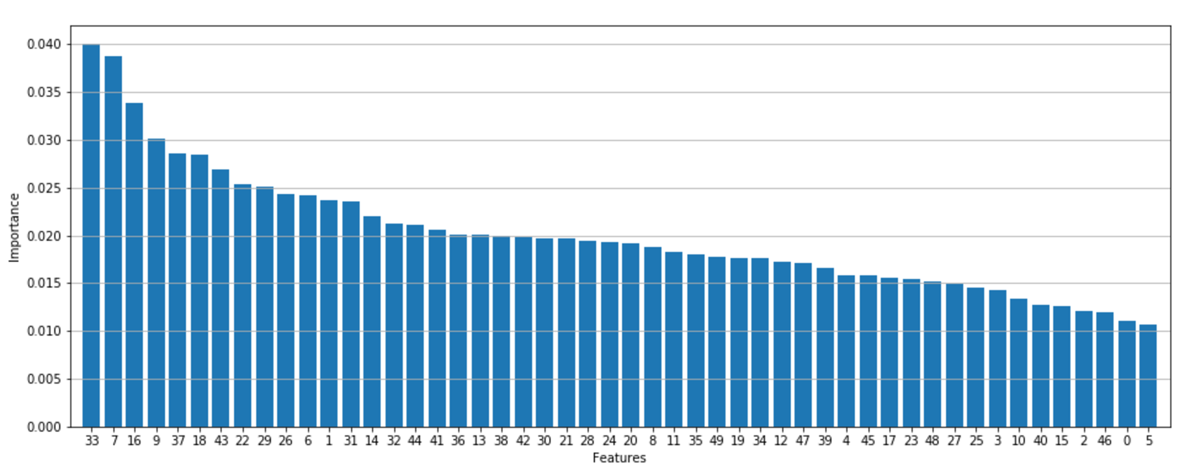 As expected, there are a few very important features, a block of features with a medium importance, and a tail containing features that have quite a low influence on the predictions. This type of plot is also useful during the analysis stage to better understand how the decision process is structured. With multidimensional datasets, it's rather difficult to understand the influence of every factor, and sometimes many important business decisions are made without a complete awareness of their potential impact. Using decision trees or random forests, it's possible to assess the "real" importance of all features and exclude all the elements under a fixed threshold. In this way, a complex decision process can be simplified and, at the same time, be partially denoised. 正如预期的那样,有几个非常重要的特征,一个中等重要性的特征块,以及一个包含对预测影响很小的特征的尾部。在分析阶段,这种类型的图对于更好地理解决策过程的结构也很有用。使用多维数据集,很难理解每个因素的影响,有时许多重要的业务决策是在没有完全意识到其潜在影响的情况下做出的。使用决策树或随机森林,可以评估所有特性的“真正”重要性,并排除固定阈值下的所有特征。这样既可以简化复杂的决策过程,又可以部分地去噪。
8.3.2 AdaBoost
Another technique is called AdaBoost (short for Adaptive Boosting) and works in a slightly different way than many other classifiers. The basic structure behind this can be a decision tree, but the dataset used for training is continuously adapted to force the model to focus on those samples that are misclassified. Moreover, the classifiers are added sequentially, so a new one boosts the previous one by improving the performance in those areas where it was not as accurate as expected.另一种技术称为AdaBoost(Adaptive Boosting的缩写),其工作方式与许多其他分类器略有不同。这背后的基本结构可以是决策树,但是用于训练的数据集不断调整,以迫使模型集中于那些错误分类的样本。此外,分类器是按顺序添加的,因此一个新的分类器通过提高在那些不像预期那样准确的领域的性能来增强前一个分类器。
At each iteration, a weight factor is applied to each sample so as to increase the importance of the samples that are wrongly predicted and decrease the importance of others. In other words, the model is repeatedly boosted, starting as a very weak learner until the maximum n_estimators number is reached. The predictions, in this case, are always obtained by majority vote.在每次迭代中,对每个样本都应用一个权重因子,以增加预测错误的样本的重要性,减少其他样本的重要性。换句话说,这个模型被反复地提升,从一个非常弱的学习者开始,直到达到最大n_estimators值。在这种情况下,预测总是通过多数票获得的。
The result is shown in the following figure:结果如下图所示:
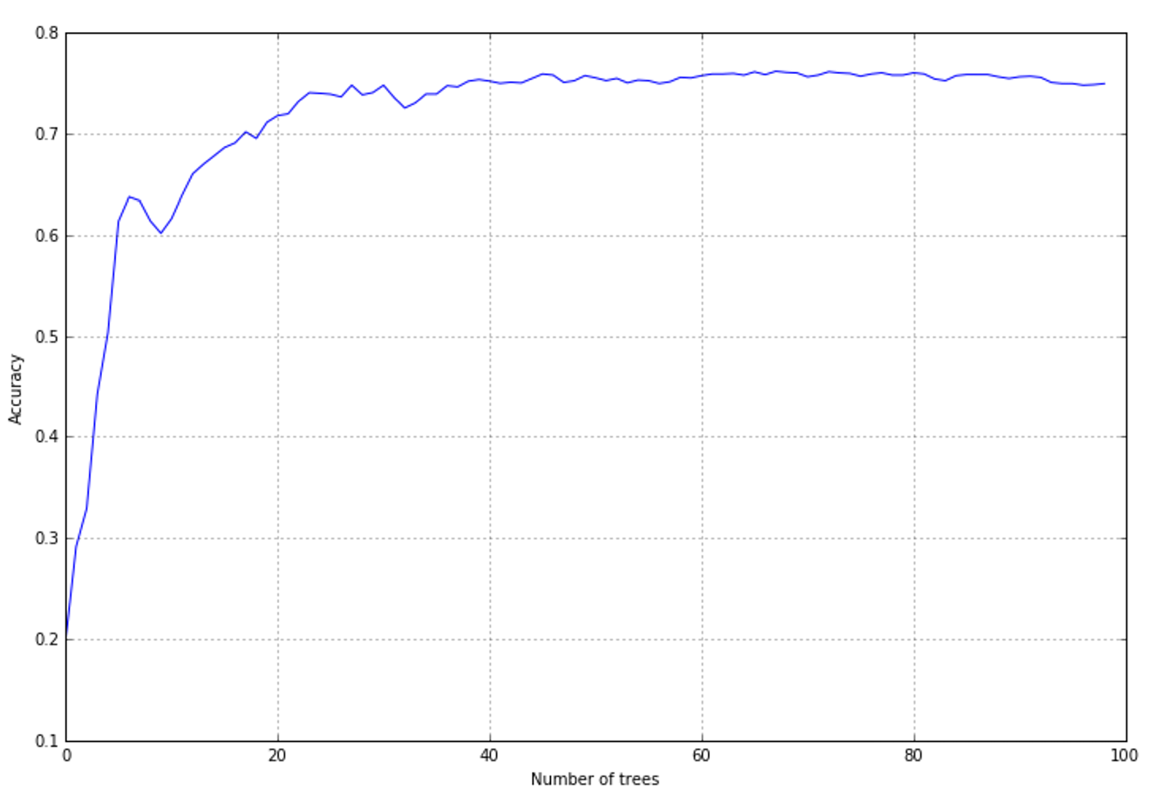 The accuracy is not so high as in the previous examples; however, it's possible to see that when the boosting adds about 20-30 trees, it reaches a stable value. A grid search on
 learning_rate could allow you to find the optimal value; however, the sequential approach in this case is not preferable. A classic random forest, which works with a fixed number of trees since the first iteration, performs better. This may well be due to the strategy adopted by AdaBoost; in this set, increasing the weight of the correctly classified samples and decreasing the strength of misclassifications can produce an oscillation in the loss function, with a final result that is not the optimal minimum point.精度不像之前的例子那么高;然而,可以看到,当增加20-30棵树时,它达到了一个稳定的值。基于learning_rate的网格搜索可以让您找到最优值;但是,在这种情况下,顺序方法并不可取。经典的随机森林从第一次迭代开始就使用固定数量的树,性能更好。这很可能是由于AdaBoost所采取的策略;在这个集合中,增加正确分类样本的权重,减少分类错误的强度,会在损失函数中产生振荡,最终结果不是优化最小值点。
In this case, a learning rate of 1.0 is the best choice, and it's easy to understand that the boosting process can be stopped after a few iterations. In the following figure, you can see a plot showing the accuracy for this dataset:在这种情况下,1.0的学习率是最好的选择,并且很容易理解在几次迭代之后可以停止提升过程。在下面的图中,您可以看到一个显示该数据集准确性的图:
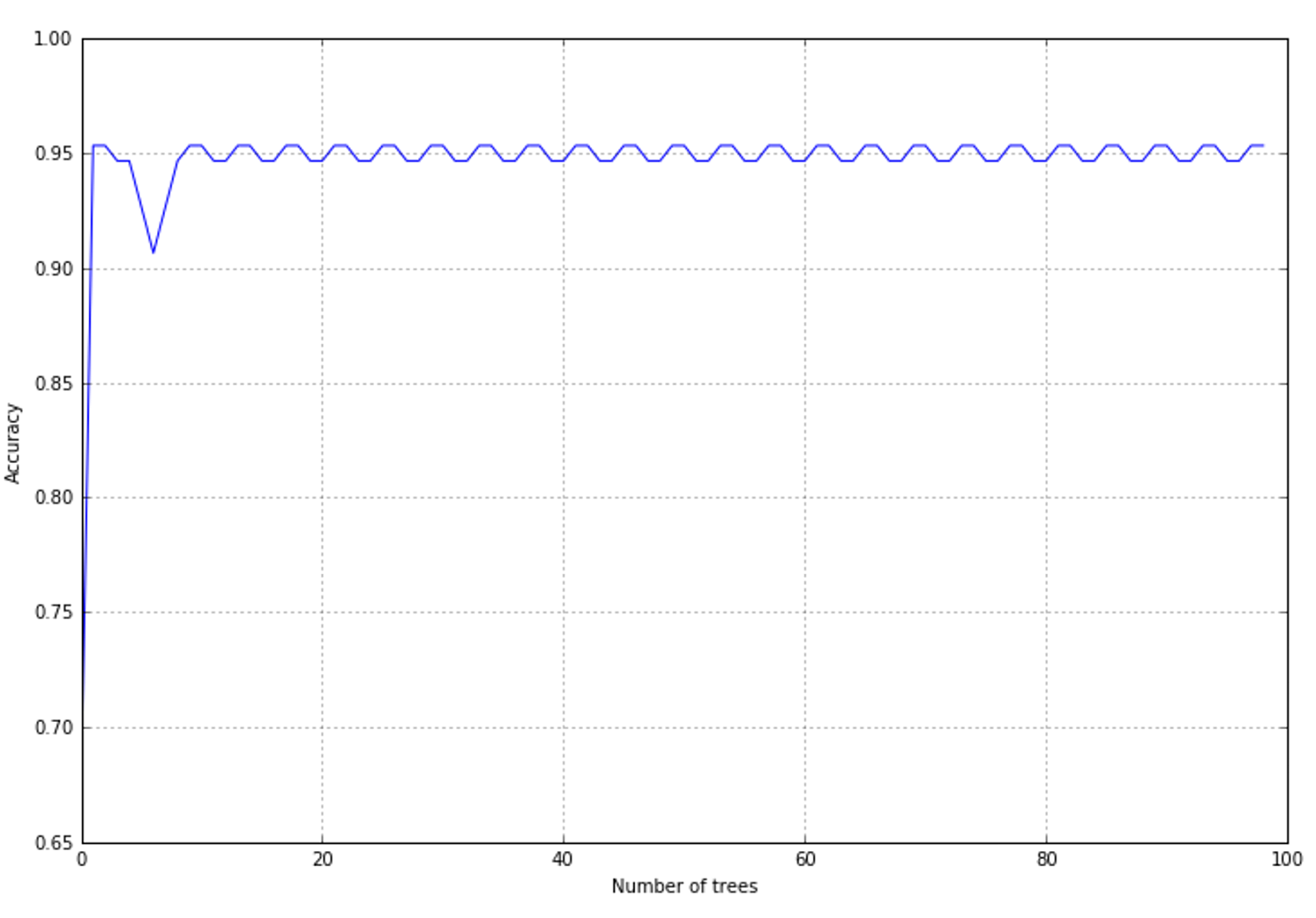 After about 10 iterations, the accuracy becomes stable (the residual oscillation can be discarded), reaching a value that is compatible with this dataset. The advantage of using AdaBoost can be appreciated in terms of resources; it doesn't work with a fully configured set of classifiers and the whole set of samples. Therefore, it can help save time when training on large datasets.经过大约10次迭代,精度变得稳定(可以丢弃残余振荡),达到与该数据集相当的值。使用AdaBoost的优势可以从资源上得到体现;它不与一组完全配置的分类器和整个示例集一起工作。因此,在大数据集上进行训练时,它可以帮助节省时间。
8.3.3 Gradient tree boosting梯度树渐进(GTB)
Gradient tree boosting is a technique that allows you to build a tree ensemble step by step with the goal of minimizing a target loss function. The generic output of the ensemble can be represented as:梯度树增强是一种技术,它允许您逐步构建树集成,目标是最小化目标损失函数。
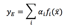
$$y_E = \sum_{i}^{}{\alpha_i f_i(\vec{x})}$$
Here, $f_i(\vec{x})$ is a function representing a weak learner. The algorithm is based on the concept of adding a new decision tree at each step so as to minimize the global loss function using the steepest gradient descent method (see Method of steepest descent, for further information):这里,$f_i(\vec{x})$表示一个弱学习器函数。该算法基于在每一步增加一个新的决策树的概念,从而使全局损失函数最小化,采用最陡梯度下降法:
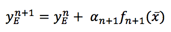
$$y_E^{n+1}=y_E^{n}+\alpha_{n+1}f_{n+1}(\vec{x})$$
After introducing the gradient, the previous expression becomes:引入梯度后,前面的表达式为:
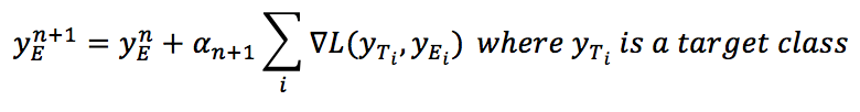
$$y_E^{n+1}=y_E^{n}+\alpha_{n+1}\sum_{i}^{}{\nabla{L(y_{T_i},y_{E_i})}} \ where \ y_{T_i} \text{ is a target class}$$
scikit-learn implements the GradientBoostingClassifier class, supporting two classification loss functions: cikit-learn实现了GradientBoostingClassifier类,支持两个分类损失函数:
- Binomial/multinomial negative log-likelihood (which is the default choice)二项式/多项式负对数似然(默认选项)
- Exponential (such as AdaBoost)指数(就如AdaBoost)
While increasing the number of estimators (parameter n_estimators), it's important to decrease the learning rate (parameter learning_rate). The optimal value cannot be easily predicted; therefore, it's often useful to perform a grid search. In our example, I've set a very high learning rate at the beginning (5.0), which converges to 0.05 when the number of estimators is equal to 100. This is not a perfect choice (unacceptable in most real cases!), and it has been made only to show the different accuracy performances. The results are shown in the following figure:在增加估计量(参数n_estimators)的同时,降低学习率(参数learning_rate)也很重要。最优值不易预测;因此,执行网格搜索通常很有用。在我们的例子中,我在开始时设置了一个非常高的学习率(5.0),当估计数等于100时,学习率收敛到0.05。这并不是一个完美的选择(在大多数实际情况下是不可接受的!),这里只是为了显示不同精度表现。结果如下图所示:

8.3.4 Voting classifier投票分类器
A very interesting ensemble solution is offered by the class VotingClassifier, which isn't an actual classifier but a wrapper for a set of different ones that are trained and evaluated in parallel. The final decision for a prediction is taken by majority vote according to two different strategies:一个非常有趣的集成解决方案是由类VotingClassifier提供的,它不是一个实际的分类器,而是对一组经过并行训练和计算的不同分类器进行包装的包装器。根据两种不同的策略,预测的最终结果由多数投票决定:
- Hard voting: In this case, the class that received the major number of votes,
$Nc(y_t)$, will be chosen:硬投票:在这种情况下,将选择获得主要票数的类$Nc(y_t)$: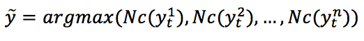
$$\hat{y}=\arg\max{(Nc(y_t^1), Nc(y_t^2), \ldots, Nc(y_t^n))}$$ - Soft voting: In this case, the probability vectors for each predicted class (for all classifiers) are summed up and averaged. The winning class is the one corresponding to the highest value:软投票:在这种情况下,对每个预测类(对于所有分类器)的概率向量求和并求平均值。获胜的类对应于最高的值:
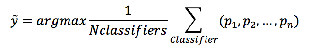
$$\hat{y}=\arg\max{(\frac{1}{N_{classifiers}}\sum_{classifier}^{}{(p_1, p_2, \ldots, p_n)})}$$
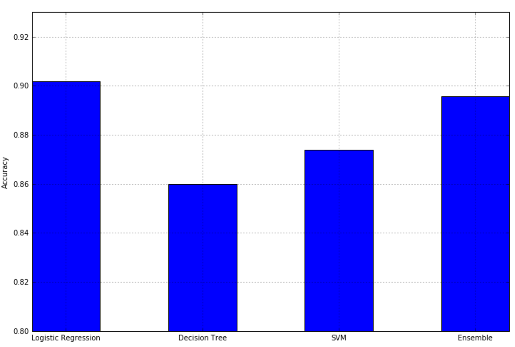
The accuracies of each single classifier and of the ensemble are plotted in the following figure:每个分类器和集合的精度如下图所示(其中Ensemble指代硬投票的VotingClassifier):
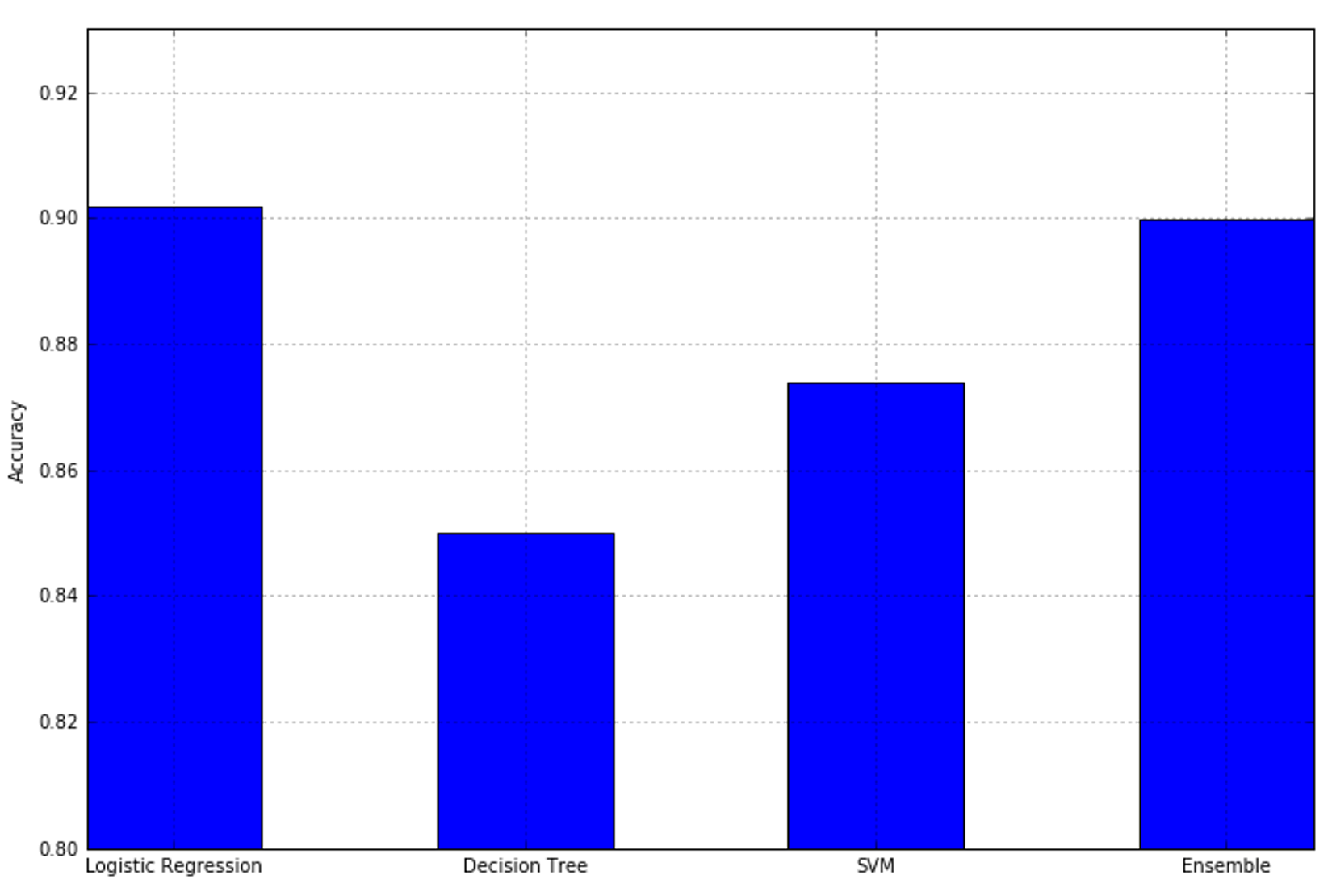 As expected, the ensemble takes advantage of the different algorithms and yields better performance than any single one. We can now repeat the experiment with soft voting, considering that it's also possible to introduce a weight vector (through the parameter
 weights) to give more or less importance to each classifier:正如预期的那样,集成利用了不同的算法,并且比任何单个算法都有更好的性能(比单独决策树算法有更好的新能)。现在我们可以重复软投票的实验,考虑到也可以引入一个权重向量(通过参数weights)来赋予每个分类器或多或少的重要性:
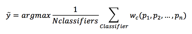
$$\hat{y}=\arg\max{(\frac{1}{N_{classifiers}}\sum_{classifier}^{}{w_c(p_1, p_2, \ldots, p_n)})}$$
The resulting plot is shown in the following figure:结果作图显示如下(其中Ensemble指代软投票的VotingClassifier):
 Weighting is not limited to the soft strategy. It can also be applied to hard voting, but in that case, it will be used to filter (reduce or increase) the number of actual occurrences.权重并不局限于软策略。它也可以应用于硬投票,但在这种情况下,它将用于过滤(减少或增加)实际发生的次数。
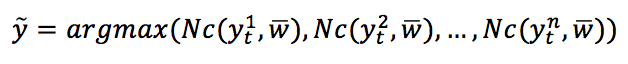
$$\hat{y}=\arg\max{(Nc(y_t^1,\vec{w}), Nc(y_t^2,\vec{w}), \ldots, Nc(y_t^n,\vec{w}))}$$
Here, $Nc(y_t,w)$ is the number of votes for each target class, each of them multiplied by the corresponding classifier weighting factor.这里,$Nc(y_t,w)$是每个目标类的投票数,每个投票数乘以相应的分类器权重因子。
A voting classifier can be a good choice whenever a single strategy is not able to reach the desired accuracy threshold; while exploiting the different approaches, it's possible to capture many microtrends using only a small set of strong (but sometimes limited) learners.当单一策略不能达到期望的精度阈值时,投票分类器是一个不错的选择;在利用不同的方法时,可以只使用一小部分强大(但有时有限)的学习器来捕捉许多微观趋势。
8.4 References参考文献
8.5 Summary总结
9 Clustering Fundamentals聚类原理
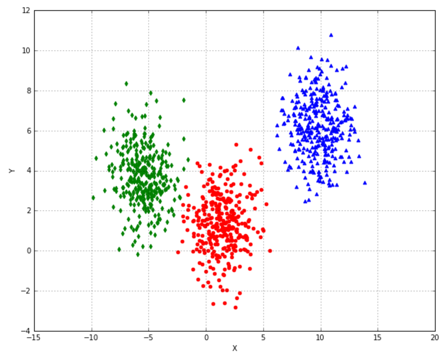
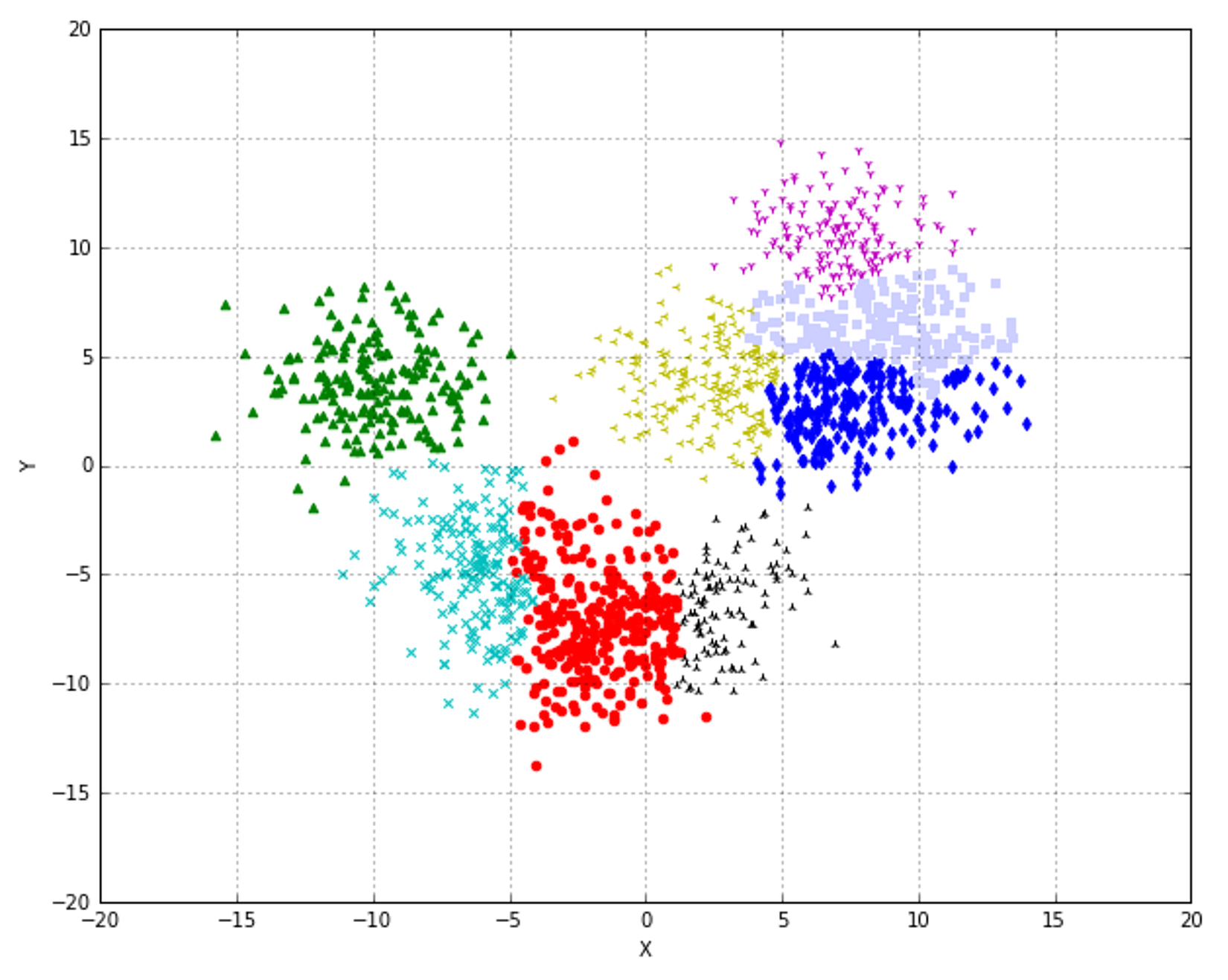
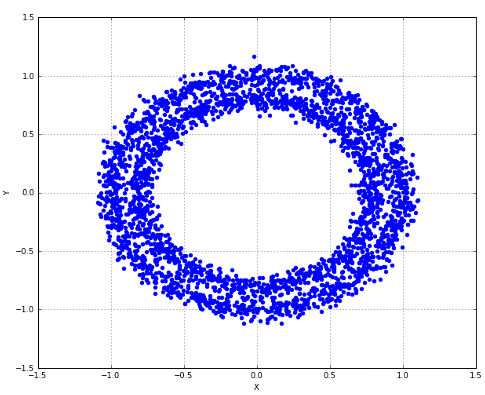
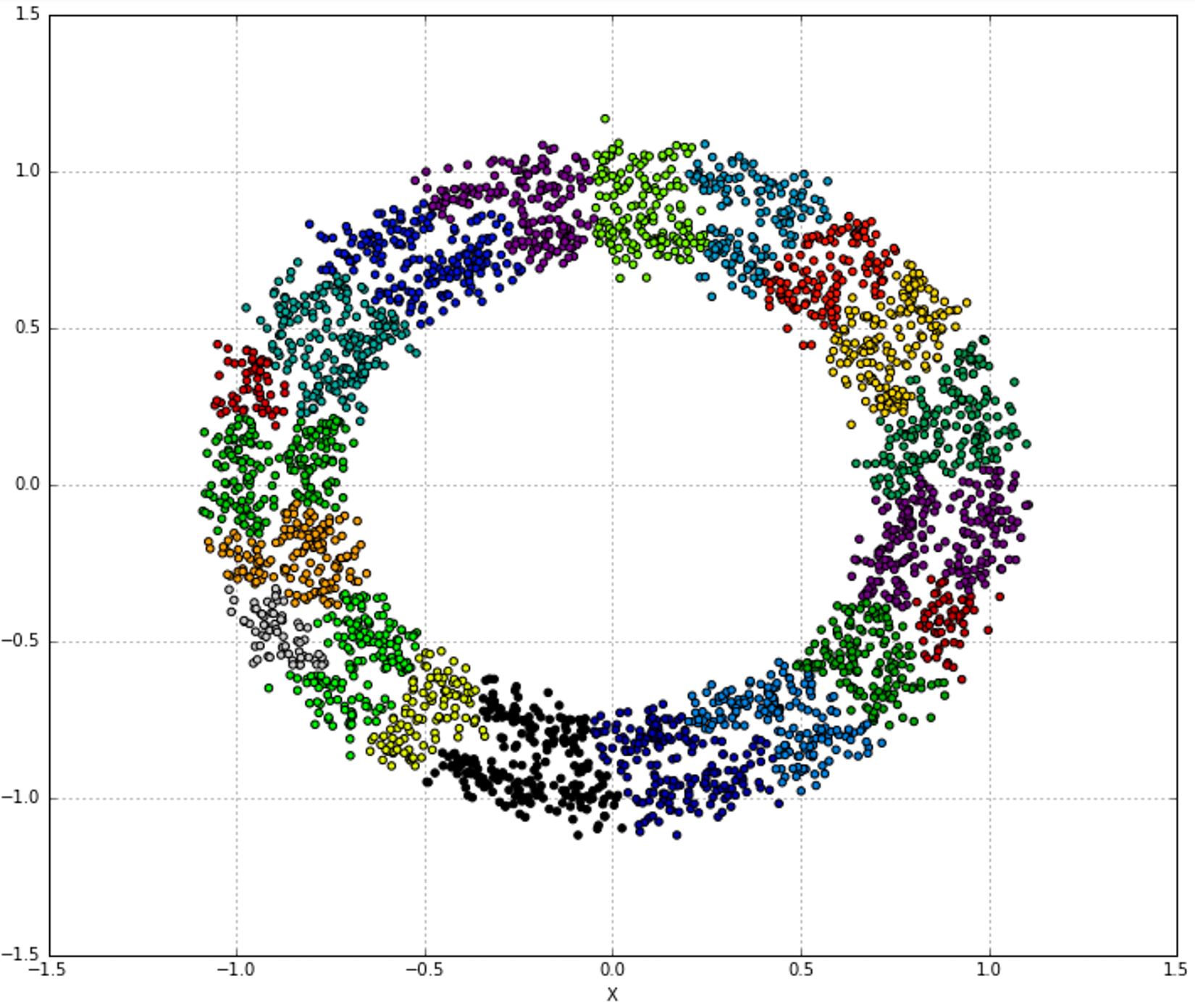
9.1 Clustering basics聚类基础
$$\mathbf{X}=\{\vec{x}_1, \vec{x}_2, \ldots, \vec{x}_n\} \quad where \ \vec{x}_i \in \mathbb{R}^m$$
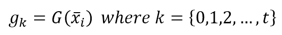
$$g_k = G(\vec{x}_i) \quad where \ k=\{0,1,2,\ldots,t\}$$

$$\vec{m}_i=F(\vec{x}_i) \quad where \ \vec{m}_i=(m_i^0, m_i^2, \ldots, m_i^t) \ and \ m_i^k \in [0,1]$$
9.1.1 K-means
$$K^{(0)}=\{\mu_1^{(0)}, \mu_2^{(0)}, \ldots, \mu_k^{(0)}\}$$
$${SS}_{W_i}=\sum_{t}^{}{\|x_t-\mu_i\|_2^2} \quad \forall i \in (1,k)$$
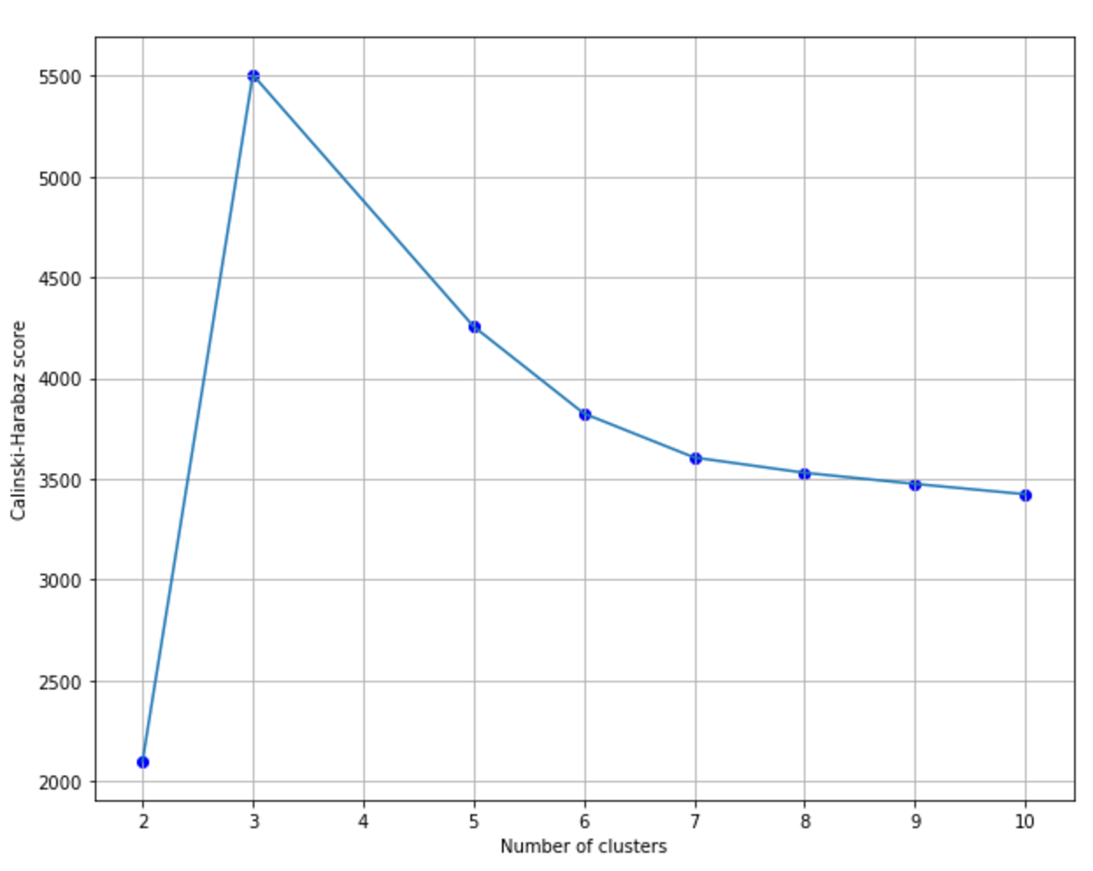
9.1.1.1 Finding the optimal number of clusters寻找最优聚类个数
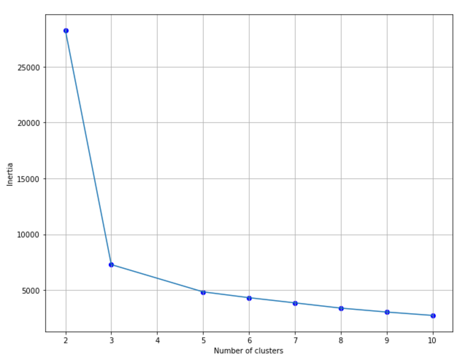
9.1.1.1.1 Optimizing the inertia优化惯性
9.1.1.1.2 Silhouette score轮廓分数
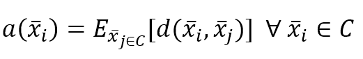
$$a(\vec{x}_i)=E_{\vec{x}_{j \in C}}[d(\vec{x}_i,\vec{x}_j)] \quad \forall \vec{x}_i \in C$$

$$b(\vec{x}_i)=E_{\vec{x}_{j \in D}}[d(\vec{x}_i,\vec{x}_j)] \quad \forall \vec{x}_i \in C \ where \ D=\arg\min\{d(C,D)\}$$
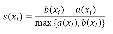
$$s(\vec{x}_i)=\frac{b(\vec{x}_i) - a(\vec{x}_i)}{\max\{a(\vec{x}_i),b(\vec{x}_i)\}}$$
9.1.1.1.3 Calinski-Harabasz index Calinski-Harabasz指数
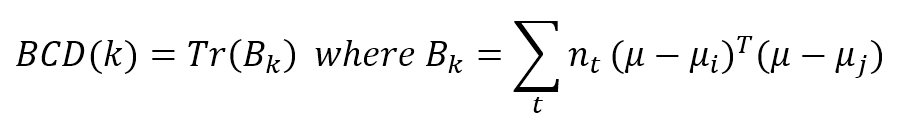
$${BCD}(k)=Tr(B_k) \quad where \ B_k = \sum_{t}^{}{n_t(\mu-\mu_i)^T(\mu-\mu_j)}$$
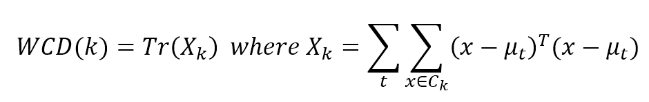
$${WCD}(k)=Tr(X_k) \quad where \ X_k = \sum_{t}^{}{\sum_{x \in C_k}^{}{(\mu-\mu_i)^T(\mu-\mu_j)}}$$
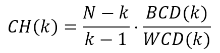
$$CH(k)=\frac{N-k}{k-1} \cdot \frac{{BCD}(k)}{{WCD}(k)}$$
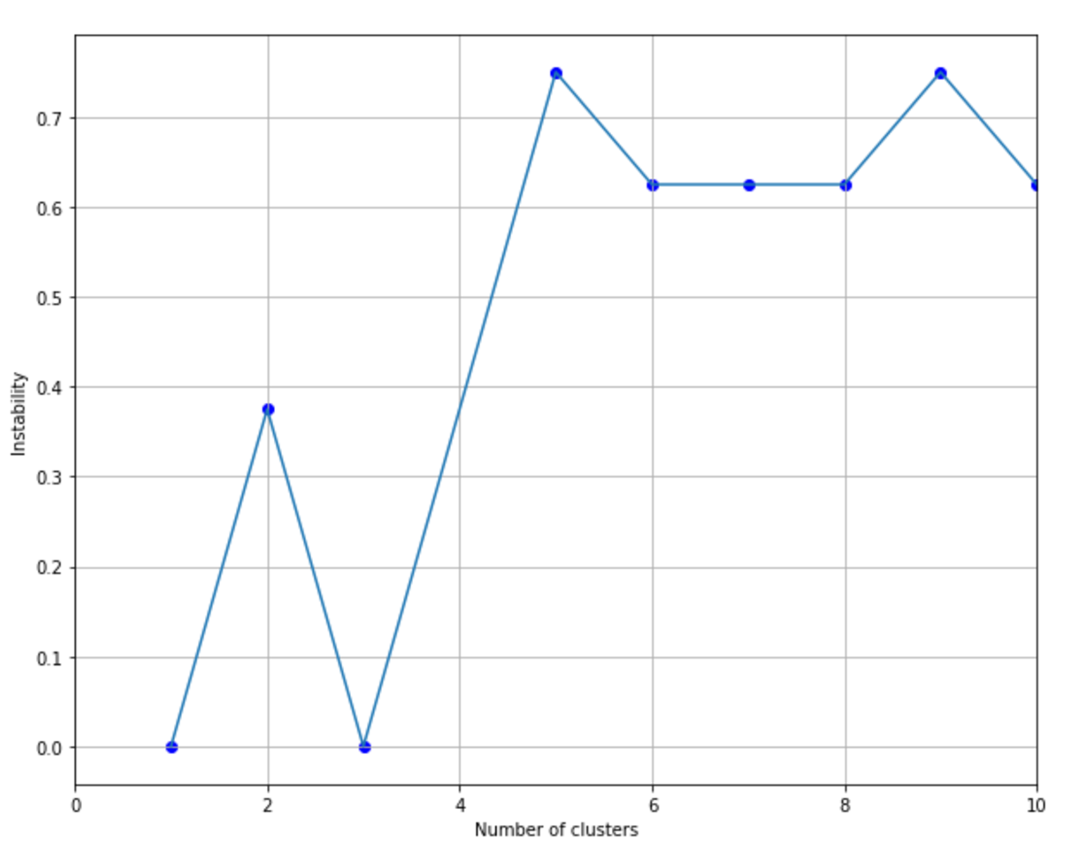
9.1.1.1.4 Cluster instability聚类不稳定性
$$X_n = \{X_n^0, X_n^1, \ldots, X_n^m\}$$
$$I(C)=E_{X_{n}^{i,j} \in X_n}\left[d\left(C(X_n^i),C(X_n^j)\right)\right]$$
9.1.2 DBSCAN
9.1.3 Spectral clustering频谱聚类
$$\mathbf{A}=\begin{pmatrix} a_{00} & \cdots & a_{0n} \\ \vdots & \ddots & \vdots \\ a_{n0} & \cdots & a_{nn} \end{pmatrix}$$
9.2 Evaluation methods based on the ground truth根据基本事实的评价方法
9.2.1 Homogeneity一致性
$$h=1-\frac{H(C|K)}{H(C)}$$
9.2.2 Completeness完整性
$$c=1-\frac{H(K|C)}{H(K)}$$
9.2.3 Adjusted rand index调整兰德指数
$$R=\frac{a+b}{\left(_2^n\right)}$$
$$AR=\frac{R-E[R]}{\max[R]-E[R]}$$
9.3 References参考文献
9.4 Summary总结
10 Hierarchical Clustering分级聚类
10.1 Hierarchical strategies分级策略
10.2 Agglomerative clustering合并聚类

$$\mathbf{X}=\{\vec{x}_1, \vec{x}_2, \ldots, \vec{x}_n\} \quad where \ \vec{x}_i \in \mathbb{R}^m$$
$$d_{Euclidean}(\vec{x}_1,\vec{x}_2)=\|\vec{x}_1-\vec{x}_2\|_2=\sqrt{\sum_{i}^{}{(x_1^i-x_2^i)^2}}$$

$$d_{Manhattan}(\vec{x}_1,\vec{x}_2)=\|\vec{x}_1-\vec{x}_2\|_2=\sum_{i}^{}{|x_1^i-x_2^i|}$$
$$d_{Cosine}(\vec{x}_1,\vec{x}_2)=1-\frac{\vec{x}_1^T \cdot \vec{x}_2}{\|\vec{x}_1\|_2\|\vec{x}_2\|_2}$$
$$\forall C_i,C_j \quad L_{ij}=\max\{d(x_a,x_b) \quad x_a \in C_i \ and \ x_b \in C_j\}$$
$$\forall C_i,C_j \quad L_{ij}=\frac{1}{|C_i||C_j|\sum_{x_a \in C_i}^{}{\sum_{x_b \in C_j}^{}{d(x_a,x_b)}}}$$
$$\forall C_i,C_j \quad L_{ij}=\sum_{x_a \in C_i}^{}{\sum_{x_b \in C_j}^{}{\|x_a-x_b\|_2^2}}$$
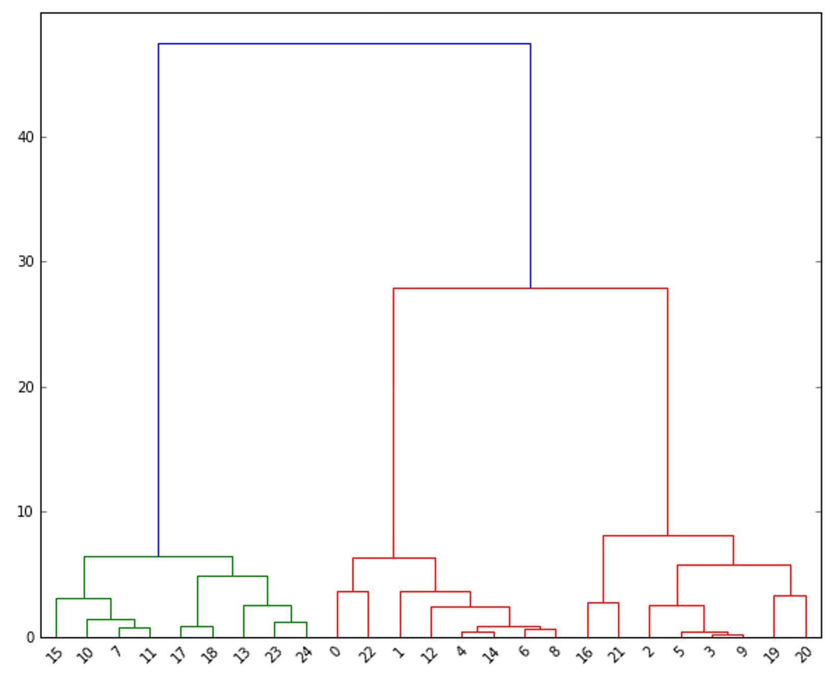
10.2.1 Dendrograms系统树图
10.2.2 Agglomerative clustering in scikit-learn 采用scikit-learn进行合并聚类
10.2.3 Connectivity constraints连通性约束
10.3 References参考文献
10.4 Summary总结
11 Introduction to Recommendation Systems推荐系统介绍
11.1 Naive user-based systems朴素基于用户系统
$$U=\{\vec{u}_1, \vec{u}_2, \ldots, \vec{u}_n\} \quad where \ \vec{u}_i \in \mathbb{R}^m$$
$$I=\{i_1, i_2, \ldots, i_m\}$$
$$g(\vec{u}) \rightarrow \{i_1, i_2, \ldots, i_k\} \quad where \ k \in (0,m)$$
$$B_R(\vec{u})=\{\vec{u}_1, \vec{u}_2, \ldots, \vec{u}_k\}$$
$$I_{Suggested}(\vec{u})=\left\{\bigcup_{i}^{}{g(\vec{u})} \quad where \ \vec{u}_i \in B_R(\vec{u})\right\}$$
11.1.1 User-based system implementation with scikit-learn在scikit-learn实现基于用户系统
$$\mathbf{M}_{UxI}=\begin{pmatrix} i_{1} & i_{2} & 0 & 0 & 0 \\ i_{15} & i_{3} & i_{12} & 0 & 0 \\ \vdots & \vdots & \vdots & \vdots & \vdots \\ i_{4} & i_{8} & i_{11} & i_{2} & i_{5} \\ i_{8} & 0 & 0 & 0 & 0 \end{pmatrix}$$
11.2 Content-based systems基于内容系统
$$I=\{\vec{l}_1, \vec{l}_2, \ldots, \vec{l}_n\} \quad where \ \vec{l}_i \in \mathbb{R}^m$$
$$d_{Minkowsky}=\left(\sum_{i}^{}{|a_i-b_i|^p}\right)^{1/p}$$
$$d_{Jaccard}=1-J(A,B)=1-\frac{|A \cap B|}{|A \cap B|}$$
11.3 Model-free (or memory-based) collaborative filtering无模型的(或基于内存的)协同过滤
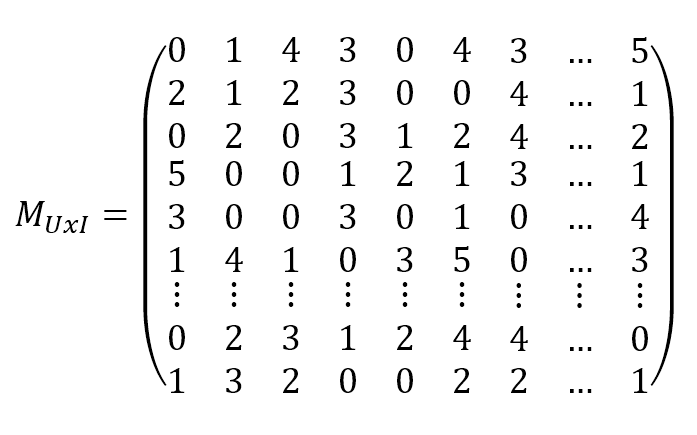
$$\mathbf{M}_{UxI}=\begin{pmatrix} 0 & 1 & 4 & 3 & 0 & 4 & 3 & \cdots & 5 \\ 2 & 1 & 2 & 3 & 0 & 0 & 4 & \cdots & 1 \\ 0 & 2 & 0 & 3 & 1 & 2 & 4 & \cdots & 2 \\ 5 & 0 & 0 & 1 & 2 & 1 & 3 & \cdots & 1 \\ 3 & 0 & 0 & 3 & 0 & 1 & 0 & \cdots & 4 \\ 1 & 4 & 1 & 0 & 3 & 5 & 0 & \cdots & 3 \\ \vdots & \vdots & \vdots & \vdots & \vdots & \vdots & \vdots & \vdots & \vdots \\ 0 & 2 & 3 & 1 & 2 & 4 & 4 & \cdots & 0 \\ 1 & 3 & 2 & 0 & 0 & 2 & 2 & \cdots & 1 \end{pmatrix}$$
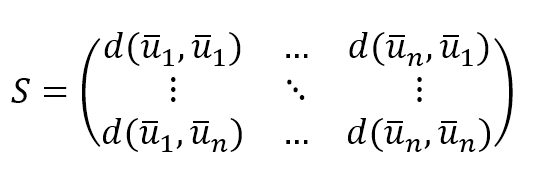
$$\mathbf{M}_{UxI}=\begin{pmatrix} d(\vec{u}_1,\vec{u}_1) & \cdots & d(\vec{u}_n,\vec{u}_1) \\ \vdots & \ddots & \vdots \\ d(\vec{u}_1,\vec{u}_n) & \cdots & d(\vec{u}_n,\vec{u}_n) \end{pmatrix}$$
11.4 Model-based collaborative filtering基于模型的协同过滤
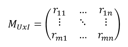
$$\mathbf{M}_{UxI}=\begin{pmatrix} r_{11} & \cdots & r_{1n} \\ \vdots & \ddots & \vdots \\ r_{m1} & \cdots & r_{mn} \end{pmatrix}$$
$$\vec{p}_i=(p_{i1}, p_{i2}, \ldots, p_{ik}) \quad where \ p_{ij} \in \mathbb{R}$$
$$\vec{q}_j=(q_{j1}, q_{j2}, \ldots, q_{jk}) \quad where \ q_{jt} \in \mathbb{R}$$
$$r_{ij}=\vec{p}_i \cdot \vec{q}_j^T$$
11.4.1 Singular Value Decomposition strategy奇异值分解(SVD)策略
$$\mathbf{M}_{UxI}=\mathbf{U}\mathbf{\Sigma}\mathbf{V}^T \quad where \ \mathbf{U} \in \mathbb{R}^{m \times t}, \mathbf{\Sigma} \in \mathbb{R}^{t \times t} \ and \ \mathbf{V} \in \mathbb{R}^{n \times n}$$
$$\mathbf{M}_{k}=\mathbf{U}_{k}\mathbf{\Sigma}_{k}\mathbf{V}_{k}^T$$
$$\left\{ \begin{aligned} \mathbf{S}_{U} & = \mathbf{U}_{k} \cdot \sqrt{\mathbf{\Sigma}_{k}}^T \\ \mathbf{S}_{I} & = \sqrt{\mathbf{\Sigma}_{k}} \cdot \mathbf{V}_{k}^T \end{aligned} \right.$$
$$\hat{r}_{ij}=E[r_i]+\mathbf{S}_{U}(i) \cdot \mathbf{S}_{I}(j)$$
11.4.2 Alternating least squares 交替最小二乘法
$$L=\sum_{(i,j)}^{}{(r_{ij}-\vec{p}_i \cdot \vec{q}_j^T)^2+\alpha(\|\vec{p}_i\|_2^2+\|\vec{q}_j\|_2^2)}$$
11.4.3 Alternating least squares with Apache Spark MLlib 用Apache Spark MLlib的交替最小二乘法
11.5 References参考文献
11.6 Summary总结
12 Introduction to Natural Language Processing自然语言处理介绍
12.1 NLTK and built-in corpora NLTK和内置语料库
12.2 The bag-of-words strategy 词袋策略
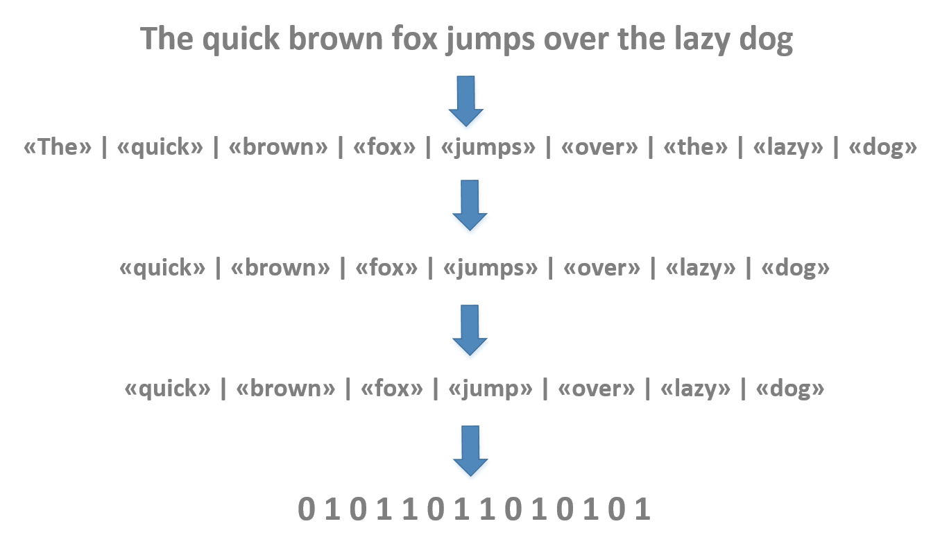
12.2.1 Tokenizing标记化
12.2.1.1 Sentence tokenizing句子标记化
12.2.1.2 Word tokenizing词标记化
12.2.2 Stopword removal停用词消除
12.2.2.1 Language detection语言识别
12.2.3 Stemming字干搜寻
12.2.4 Vectorizing向量化
12.2.4.1 Count vectorizing计数向量化
12.2.4.1.1 N-grams
12.2.4.2 Tf-idf vectorizing Tf-idf向量化
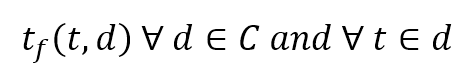
$$t_f(t,d) \quad \forall d \in C \ and \ forall t \in d$$
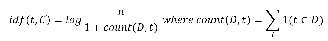
$$idf(t,C)=\log{\frac{n}{1+{count}(D,t)}} \quad where \ {count}(D,t)=\sum_{i}^{}{1(t \in D)}$$
$$t_f \cdot idf(t,d,C)=t_f(t,d)idf(t,C)$$
12.3 A sample text classifier based on the Reuters corpus基于路透社语料库的文本分类器示例
12.4 References参考文献
12.5 Summary总结
13 Topic Modeling and Sentiment Analysis in NLP自然语言处理(NLP)中的主题建模和情绪分析
13.1 Topic modeling主题建模
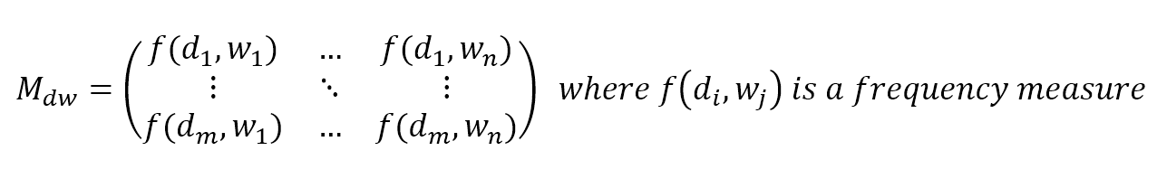
$$\mathbf{M}_{dw}=\begin{pmatrix} f(d_1,w_1) & \cdots & f(d_1,w_n) \\ \vdots & \ddots & \vdots \\ f(d_m,w_1) & \cdots & f(d_m,w_n) \end{pmatrix} \quad where f(d_i,w_j) \text{ is a frequency measure}$$
13.1.1 Latent semantic analysis潜在语义分析

$$\mathbf{M}_{UxI}=\mathbf{U}\mathbf{\Sigma}\mathbf{V}^T \quad where \ \mathbf{U} \in \mathbb{R}^{m \times t}, \mathbf{\Sigma} \in \mathbb{R}^{t \times t} \ and \ \mathbf{V} \in \mathbb{R}^{n \times n}$$

$$\mathbf{M}_{k}=\mathbf{U}_{k}\mathbf{\Sigma}_{k}\mathbf{V}_{k}^T$$
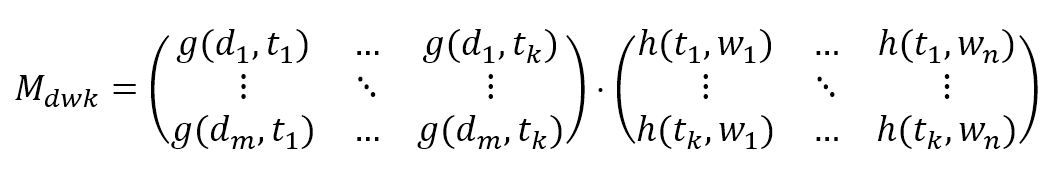
$$\mathbf{M}_{dwk}=\begin{pmatrix} g(d_1,t_1) & \cdots & g(d_1,t_k) \\ \vdots & \ddots & \vdots \\ g(d_m,t_1) & \cdots & g(d_m,t_k) \end{pmatrix} \cdot \begin{pmatrix} h(t_1,w_1) & \cdots & h(t_1,w_n) \\ \vdots & \ddots & \vdots \\ h(t_k,w_1) & \cdots & h(t_k,w_n) \end{pmatrix}$$
$$\mathbf{M}_{dwk}=\mathbf{M}_{dtk} \cdot \mathbf{M}_{twk}$$
$$d_i=\sum_{j=1}^{k}{g(d_i,t_k)}$$
$$t_i \approx \sum_{j=1}^{r}{h_{ji}w_{j}}$$
$$\mathbf{M}_{twk}=\mathbf{V}_{k}$$
$$\mathbf{M}_{dtk}=\mathbf{U}_{k}\mathbf{\Sigma}_{k}$$
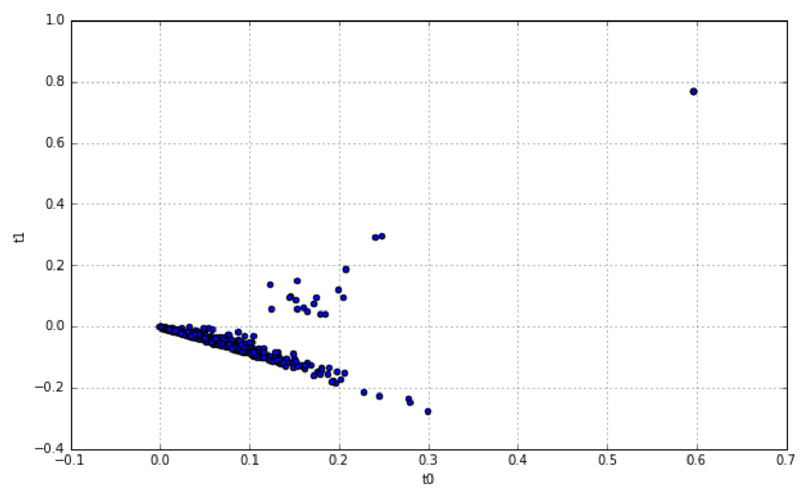
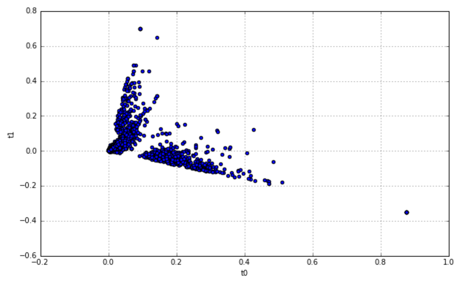
13.1.2 Probabilistic latent semantic analysis概率潜在语义分析
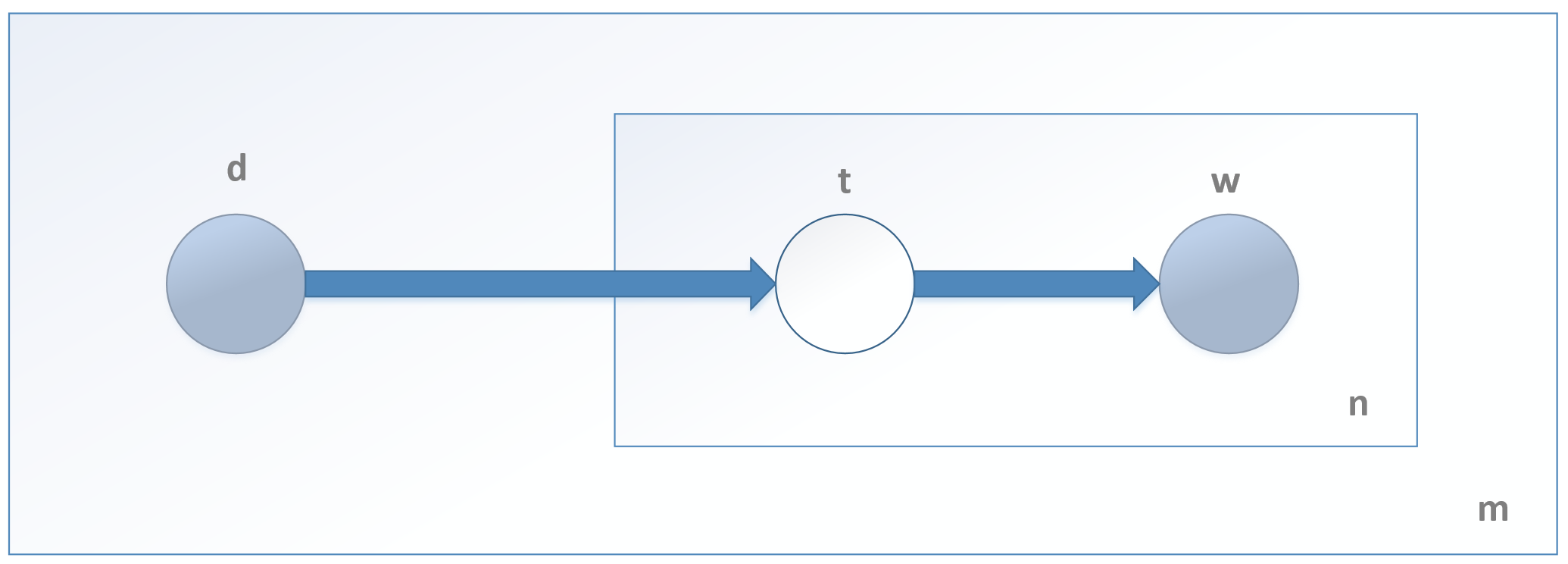
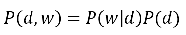
$$P(d,w)=P(w|d)P(d)$$
$$P(w|d)=\sum_{i=1}^{k}{P(w|t_i)P(t_i|d)}$$
$$P(d,w)=\sum_{i=1}^{k}{P(t_i)P(w|t_i)P(d|t_i)}$$
$$L=\sum_{d}^{}{\sum_{w}^{}{M_{dw}(d,w) \cdot \log{P(d,w)}}}$$
$$L=\sum_{d}^{}{\sum_{w}^{}{\left(M_{dw}(d,w) \cdot \log{P(d)}+M_{dw}(d,w) \cdot \log{\sum_{k}^{}{P(t_k|d)P(w|t_k)}}\right)}}$$
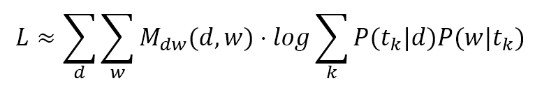
$$L \approx \sum_{d}^{}{\sum_{w}^{}{\left(M_{dw}(d,w) \cdot \log{\sum_{k}^{}{P(t_k|d)P(w|t_k)}}\right)}}$$
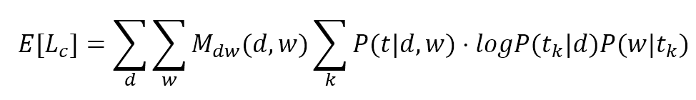
$$E[L_c] = \sum_{d}^{}{\sum_{w}^{}{\left(M_{dw}(d,w) \sum_{k}^{}{P(t|d,w) \cdot \log{(P(t_k|d)P(w|t_k))}}\right)}}$$
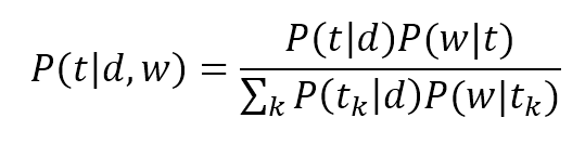
$$P(t|d,w)=\frac{P(t|d)P(w|t)}{\sum_{k}^{}{P(t_k|d)P(w|t_k)}}$$
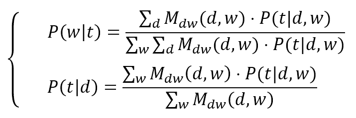
$$\left\{ \begin{aligned} P(w|t) & = \frac{\sum_{d}^{}{(M_{dw}(d,w)) \cdot P(t|d,w)}}{\sum_{w}^{}{\sum_{d}^{}{(M_{dw}(d,w))}} \cdot P(t|d,w)} \\ P(t|w) & = \frac{\sum_{w}^{}{(M_{dw}(d,w)) \cdot P(t|d,w)}}{\sum_{w}^{}{M_{dw}(d,w)}} \end{aligned} \right.$$
13.1.3 Latent Dirichlet Allocation潜在狄利克雷定位
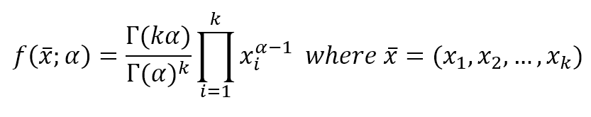
$$f(\vec{x};\alpha)=\frac{\Gamma(k \alpha)}{\Gamma(k \alpha)^k} \prod_{i=1}^{k}{x_i^{\alpha-1}} \quad where \ \vec{x}=(x_1,x_2,\ldots,x_k)$$
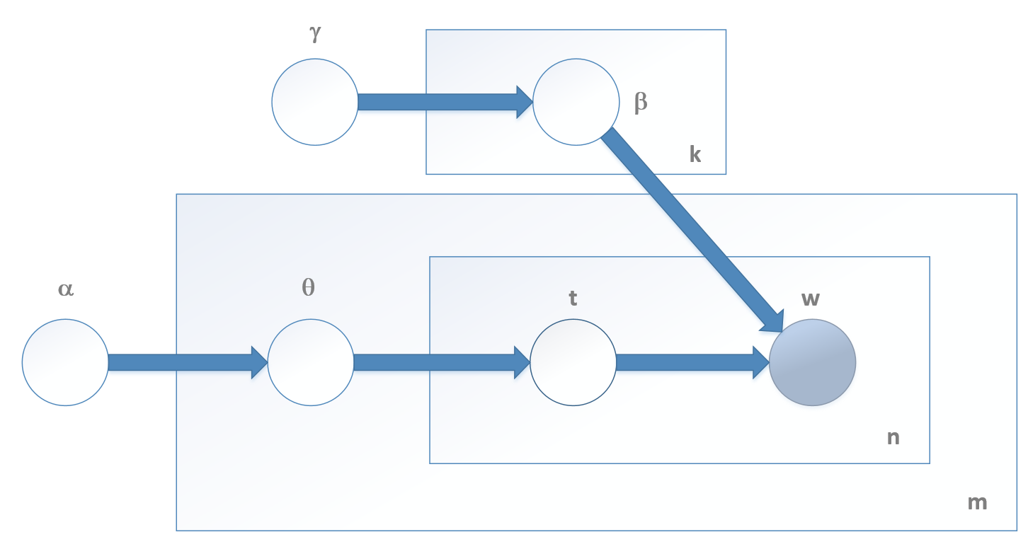
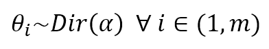
$$\theta_i \sim Dir(\alpha) \quad \forall i \in (1,m)$$
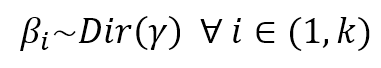
$$\beta_i \sim Dir(\gamma) \quad \forall i \in (1,k)$$
$$z_{dw} \sim Categorical(\theta_d)$$
$$w_{wj} \sim Categorical(\beta_{z_{dw}})$$
$$p(\vec{z},\theta,\beta|\vec{w},\alpha,\gamma)=\frac{p(\vec{z},\theta,\beta|\alpha,\gamma)}{p(\vec{w}|\alpha,\gamma)}$$
$$p(\theta,\vec{z},\vec{w}|\alpha,\gamma)=p(\theta|\alpha)\prod_{i}^{}{p(z_i|\theta)p(w_i|z_i,\gamma)}$$
$$p(\vec{w}|\alpha,\gamma)=\int p(\theta|\alpha)\left(\prod_{i}^{}{\sum_{z_i}^{}{p(z_i|\theta)p(w_i|z_i,\gamma)}}\right) \ d \theta$$
13.2 Sentiment analysis语义分析
13.2.1 VADER sentiment analysis with NLTK用NLTK的VADER语义分析
$${Compound}=\frac{\sum_{i}^{}{Sentiment(w_i)}}{\sqrt{(\sum_{i}^{}{Sentiment(w_i)})^2 + \alpha}}$$
13.3 References参考文献
13.4 Summary总结
14 A Brief Introduction to Deep Learning and TensorFlow深度学习和TensorFlow简介
14.1 Deep learning at a glance深度学习一瞥
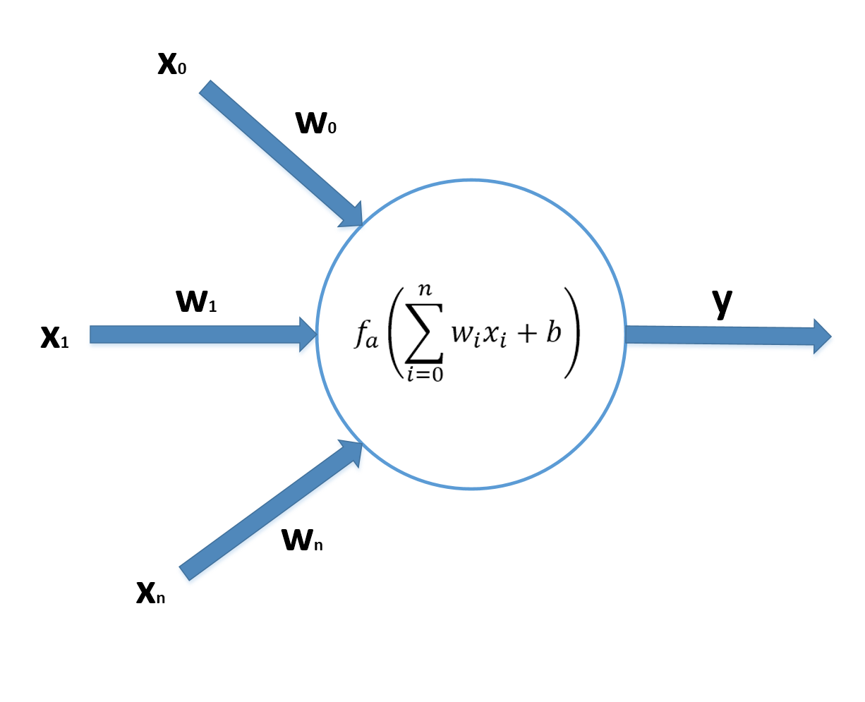
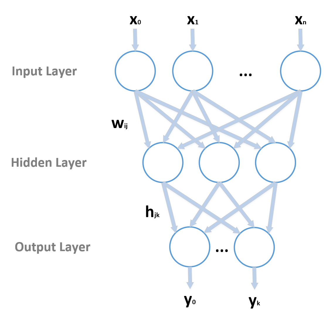
14.1.1 Artificial neural networks人工神经网络
$$\vec{y}=f(\vec{x})$$
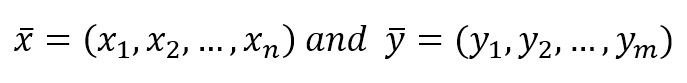
$$\vec{x}=(x_1, x_2, \ldots, x_n) \ and \ \vec{y}=(y_1, y_2, \ldots, y_m)$$
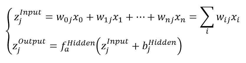
$$\left\{ \begin{aligned} z_j^{Input} & = w_{0j}x_0 + w_{1j}x_1 + \cdots + w_{nj}x_n = \sum_{i}^{}{w_{ij}x_i} \\ z_j^{Output} & = f_a^{Hidden}\left(z_j^{Input} + b_j^{Hidden}\right) \end{aligned} \right.$$
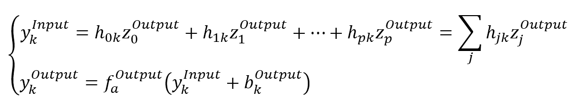
$$\left\{ \begin{aligned} y_k^{Input} & = h_{0k}z_j^{Output} + h_{1k}z_1^{Output} + \cdots + h_{pk}z_p^{Output} = \sum_{j}^{}{h_{jk}z_j^{Output}} \\ y_k^{Output} & = f_a^{Output}\left(y_k^{Input} + b_k^{Output}\right) \end{aligned} \right.$$
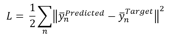
$$L=\frac{1}{2}\sum_{n}^{}{\|\vec{y}_n^{Predicted}-\vec{y}_n^{Target}\|_2^2}$$
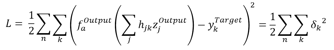
$$\begin{align}
L & = \frac{1}{2}\sum_{n}^{}{\sum_{k}^{}{\left(f_a^{Output}\left(\sum_{j}^{}{h_{jk}z_j^{Output}}\right)-y_k^{Target}\right)^2}} \\
& = \frac{1}{2}\sum_{n}^{}{\sum_{k}^{}{\delta_k^2}}
\end{align}$$
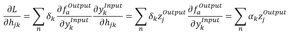
$$\begin{align}
\frac{\partial{L}}{\partial{h_{jk}}} & = \sum_{n}^{}{\left(\delta_k  \cdot \frac{\partial{f_a^{Output}}}{\partial{y_k^{Input}}} \cdot \frac{\partial{y_k^{Input}}}{\partial{h_{jk}}}\right)} \\
& = \sum_{n}^{}{\left(\delta_k  \cdot z_j^{Output} \frac{\partial{f_a^{Output}}}{\partial{y_k^{Input}}} \right)}  \\
& = \sum_{n}^{}{\left(\alpha_k  \cdot z_j^{Output} \right)}
\end{align}$$
$$\begin{align}
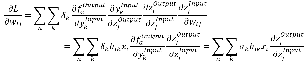
\frac{\partial{L}}{\partial{w_{ij}}} & = \sum_{n}^{}{\sum_{k}^{}{\left(\delta_k \cdot \frac{\partial{f_a^{Output}}}{\partial{y_k^{Input}}} \cdot \frac{\partial{y_k^{Input}}}{\partial{z_j^{Output}}} \cdot \frac{\partial{z_j^{Output}}}{\partial{z_j^{Intput}}} \cdot \frac{\partial{z_j^{Intput}}}{\partial{w_{ij}}}\right)}} \\
& = \sum_{n}^{}{\sum_{k}^{}{\left(\delta_k \cdot h_{jk} \cdot x_i \cdot \frac{\partial{f_a^{Output}}}{\partial{y_k^{Input}}} \cdot \frac{\partial{z_j^{Output}}}{\partial{z_j^{Intput}}}\right)}} \\
& = \sum_{n}^{}{\sum_{k}^{}{\left(\delta_k \cdot h_{jk} \cdot x_i \cdot \frac{\partial{z_j^{Output}}}{\partial{z_j^{Intput}}}\right)}}
\end{align}$$
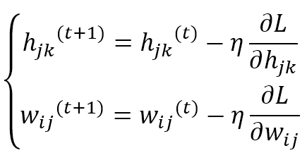
$$\left\{ \begin{aligned} h_{jk}^{(t+1)} & = h_{jk}^{(t)} - \eta \frac{\partial{L}}{\partial{h_{jk}}} \\ w_{ij}^{(t+1)} & = w_{ij}^{(t)} - \eta \frac{\partial{L}}{\partial{w_{ij}}} \end{aligned} \right.$$
14.1.2 Deep architectures深度结构
14.1.2.1 Fully connected layers全连接层
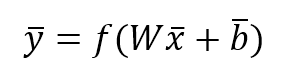
$$\vec{y}=f(W \vec{x}+\vec{b})$$
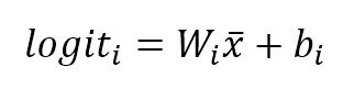
$$logit_i=W_i \vec{x}+b_i$$
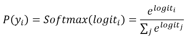
$$P(y_i)=Softmax(logit_i)=\frac{e^{logit_i}}{\sum_{j}^{}{e^{logit_j}}}$$
14.1.2.2 Convolutional layers卷积层
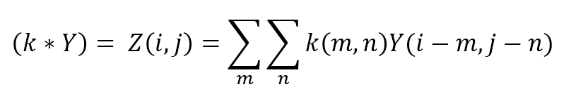
$$(k * Y) = Z(i,j)=\sum_{m}^{}{\sum_{n}^{}{\left(k(m,n)Y(i-m,j-n)\right)}}$$
14.1.2.3 Dropout layers 丢弃层
14.1.2.4 Recurrent neural networks递归神经网络
14.2 A brief introduction to TensorFlow TensorFlow简介
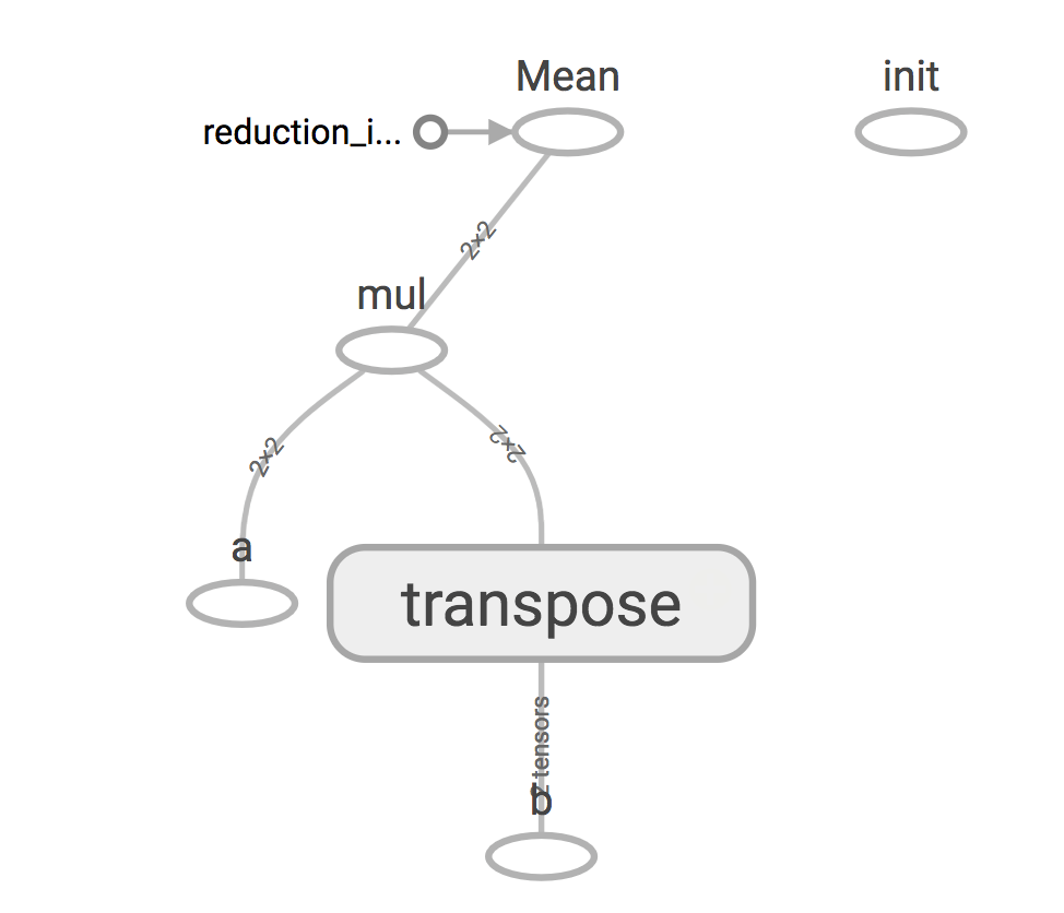
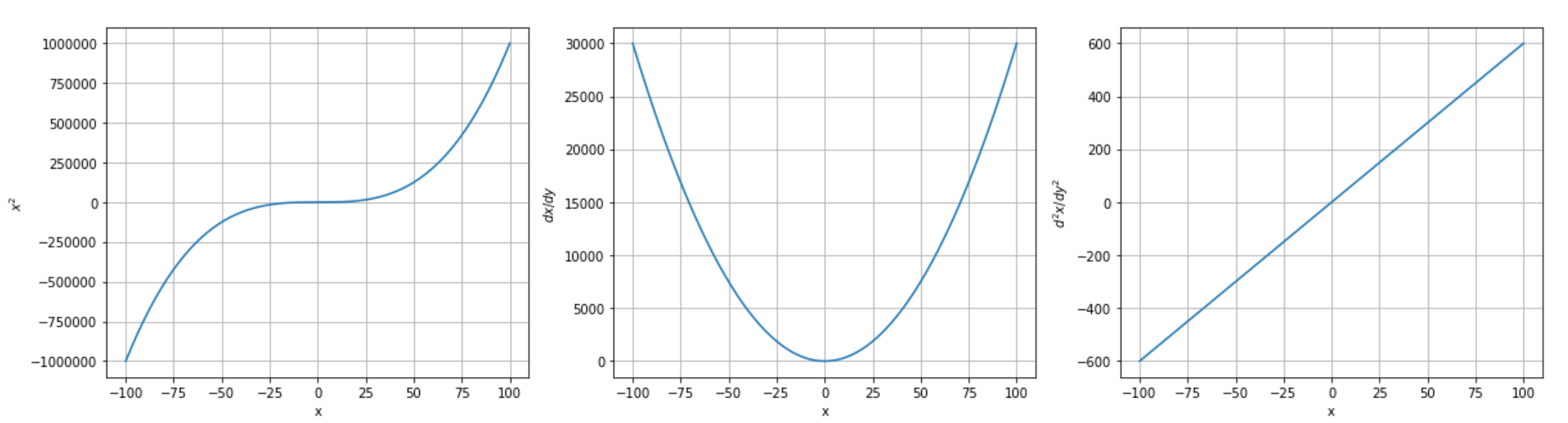
14.2.1 Computing gradients计算梯度
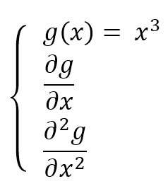
$$\left\{ \begin{aligned} & g(x) = x^3 \\ & \frac{\partial{g}}{\partial{x}} \\ & \frac{\partial^2{g}}{\partial{x}^2} \end{aligned} \right.$$
14.2.2 Logistic regression逻辑回归
14.2.3 Classification with a multi-layer perceptron用多层感知器进行分类
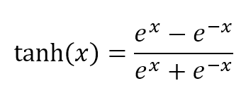
$$tanh(x)=\frac{e^x-e^{-x}}{e^x+e^{-x}}$$
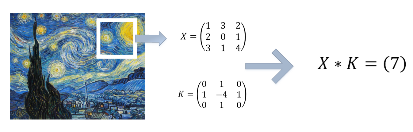
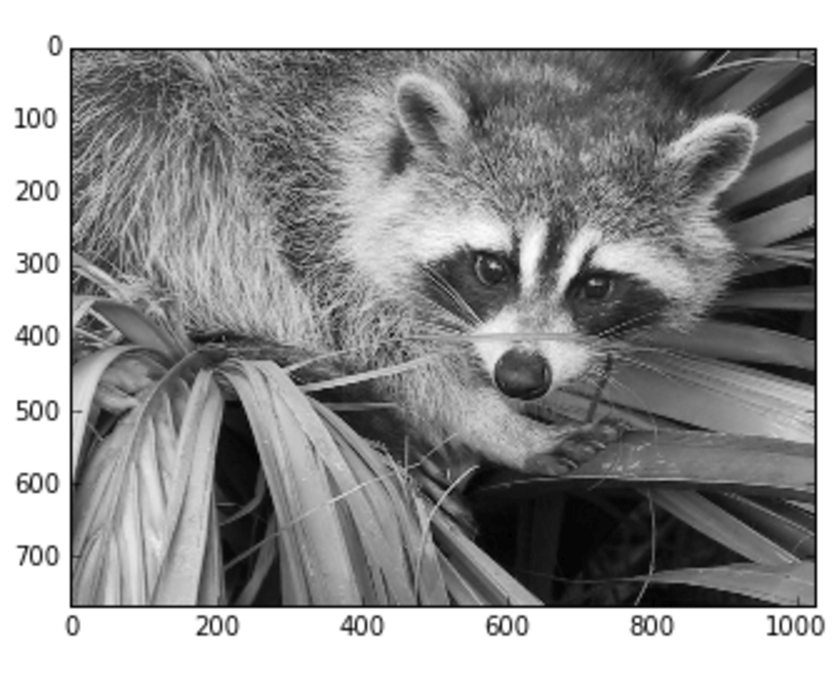
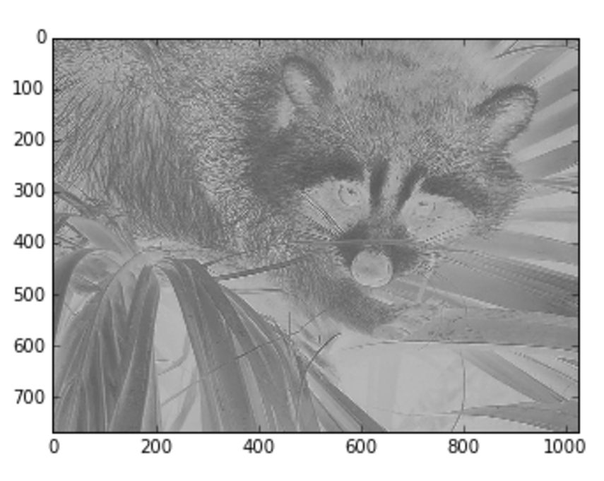
14.2.4 Image convolution图片卷积
14.3 A quick glimpse inside Keras快速一瞥Keras的内部
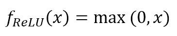
$$f_{ReLU}(x)=\max(0,x)$$
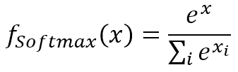
$$f_{Softmax}(x)=\frac{e^x}{\sum_{i}^{}{e^{x_i}}}$$
14.4 References参考文献
14.5 Summary总结
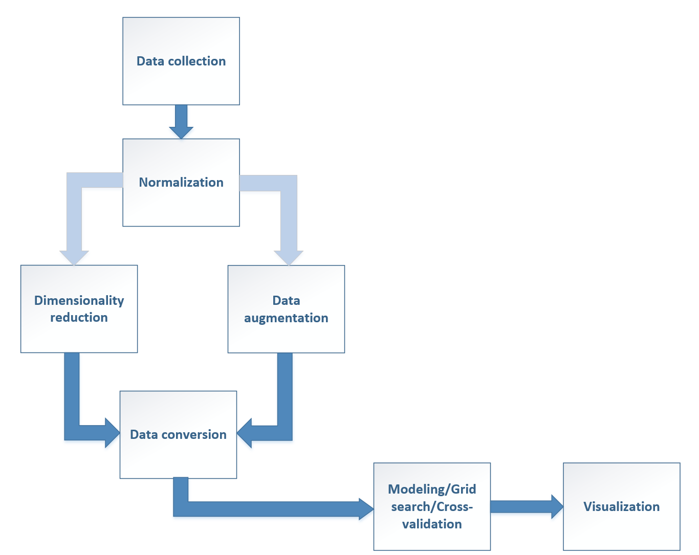
15 Creating a Machine Learning Architecture创建机器学习结构
15.1 Machine learning architectures机器学习结构