核方法kernel_method
$$
方程latex参考skearn、分类、定义等框架参考维基。
本质上来说,核函数就是一个内积函数,定义了一个内积空间。因此核函数和普通内积一样,都可以看成是衡量两个向量相似程度的函数。
根据公式2,核函数可分解为两个行向量$\vec{x}_1$和$\vec{x}_1$的转换到另一空间$\mathcal{V}$后的向量$\varphi (\vec {x}_1)$和$\varphi (\vec {x}_1)$的乘积,除非采用线性核函数,否则$\varphi (\vec {x}_1)$一定将$\vec{x}_1$进行了非线性的转换,所以核技巧可以对数据进行非线性转换。
采用了核技巧的KernelPCA可以利用$\varphi (\vec {x})$对数据矩阵进行非线性转换,再行降维(当然,PCA、KernelPCA、SparsePCA等均有n_components参数用于设置维度转换后的维度数,并没有要求一定小于m,像所有PCA一样,既可升维又可降维)。
采用了核技巧的SVM可以利用$\varphi (\vec {x})$对数据矩阵进行非线性转换,转换后特征矩阵将易于划分。同时核函数$k(\vec {x}_i ,\vec {x})$将用于训练数据集以外数据的预测。比如,对于SVC其实就是根据公式2,公式2中另一参数根据另一优化得到。详情参阅博文支持向量机svm之数学原理。
In machine learning, kernel methods are a class of algorithms for pattern analysis, whose best known member is the support vector machine (SVM). The general task of pattern analysis is to find and study general types of relations (for example clusters, rankings, principal components, correlations, classifications) in datasets. In its simplest form, the kernel trick means transforming data into another dimension that has a clear dividing margin between classes of data.[1] For many algorithms that solve these tasks, the data in raw representation have to be explicitly transformed into feature vector representations via a user-specified feature map: in contrast, kernel methods require only a user-specified kernel, i.e., a similarity function over pairs of data points in raw representation.在机器学习中,核方法是模式分析的一类算法,其最广为人知的是用于支持向量机(SVM)。模式分析的一般任务是发现和研究数据集中关系的一般类型(例如集群、排名、主成分、相关性、分类)。在最简单的形式中,核技巧意味着将数据转换为另一个维度,数据类之间在该维度有明显的分隔。对于许多解决这些任务的算法,原始表示中的数据必须通过用户指定的feature map显式地转换为feature vector表示:相比之下,核方法只需要用户指定的核,即,是对原始表示的数据点对的一种相似性函数。
Kernel methods owe their name to the use of kernel functions, which enable them to operate in a high-dimensional, implicit feature space without ever computing the coordinates of the data in that space, but rather by simply computing the inner products between the images of all pairs of data in the feature space. This operation is often computationally cheaper than the explicit computation of the coordinates. This approach is called the "kernel trick"[2]. Kernel functions have been introduced for sequence data, graphs, text, images, as well as vectors.核方法命名源于内核函数的使用,这使他们在一个高维、隐式特征空间下,不计算在这个空间的坐标数据,而是通过简单计算特征空间下全部数据对的图像之间的内积。这一操作通常较显式计算坐标更不消耗算力。这一方法叫做核技巧。为序列数据、图像、文本、照片还有向量引入核函数。
Algorithms capable of operating with kernels include the kernel perceptron, support vector machines (SVM), Gaussian processes, principal components analysis (PCA), canonical correlation analysis, ridge regression, spectral clustering, linear adaptive filters and many others. Any linear model can be turned into a non-linear model by applying the kernel trick to the model: replacing its features (predictors) by a kernel function[3]. 可采用核操作的算法包括:核感知机、支持向量机(SVM)、高斯过程、主成分分析(PCA)、典型相关分析、岭回归、谱聚类、线性自适应滤波器等等。对任何线性模型施加核技巧可将之转化成非线性模型:用核函数替代增加(维基原文是替代,我认为核函数相当于一个特征列,替代将浪费大量信息。)其特征(或者预测变量)。
Most kernel algorithms are based on convex optimization or eigenproblems and are statistically well-founded. Typically, their statistical properties are analyzed using statistical learning theory (for example, using Rademacher complexity).大多数核算法都是基于凸优化或特征问题的,并且具有良好的统计基础。通常,使用统计学习理论(例如,使用Rademacher复杂度)分析它们的统计特性。
1 Motivation and informal explanation
Kernel methods can be thought of as instance-based learners: rather than learning some fixed set of parameters corresponding to the features of their inputs, they instead "remember" the
$i$
-th training example
$(\vec {x} _{i},\vec{y}_{i})$
and learn for it a corresponding weight
$w_{i}$
. Prediction for unlabeled inputs, i.e., those not in the training set, is treated by the application of a similarity function
$k$
, called a kernel, between the unlabeled input
$\vec {x}'$
and each of the training inputs
$\vec {x} _{i}$
. For instance, a kernelized binary classifier typically computes a weighted sum of similarities:核方法可以看作是基于实例的学习者:它们不是学习与输入特性相对应的固定参数集,而是“记住”第$i$个训练样本$(\vec {x} _{i},\vec{y}_{i})$并学习其对应的参数$w_{i}$。未标记输入的预测,即在未标记的输入$\vec {x}'$和每个训练输入$\vec {x} _{i}$之间(既然叫输入,那么$\vec {x}'$和$\vec {x} _{i}$是行向量),应用一个称为核的相似度函数$k$来处理那些不在训练集中的输入。例如,核化的二分类器通常计算相似度的加权合计:
$${\hat {y}}=\operatorname {sgn} \sum _{i=1}^{n}w_{i}y_{i}k(\vec {x} _{i},\vec {x}' ) \tag{1}$$
where:其中:
${\hat {y}}\in \{-1,+1\}$is the kernelized binary classifier's predicted label for the unlabeled input$\vec {x}'$whose hidden true label$y$is of interest;${\hat {y}}\in \{-1,+1\}$是核化二分类器的预测标签,对于未被标记的输入$\vec {x}'$,我们关心其未知的标签$y$;$k\colon {\mathcal {X}}\times {\mathcal {X}}\to \mathbb {R}$is the kernel function that measures similarity between any pair of inputs$\vec {x} ,\vec {x}' \in {\mathcal {X}}$;$k\colon {\mathcal {X}}\times {\mathcal {X}}\to \mathbb {R}$是测量任意输入对$\vec {x} ,\vec {x}' \in {\mathcal {X}}$之间相似度的核函数;- the sum ranges over the n labeled examples
$\{(\vec {x} _{i},\vec{y}_{i})\}_{i=1}^{n}$in the classifier's training set, with$y_{i}\in \{-1,+1\}$;求和应包括分类器中全部n个标记了的样本$\{(\vec {x} _{i},\vec{y}_{i})\}_{i=1}^{n}$,其中$y_{i}\in \{-1,+1\}$; - the
$w_{i}\in \mathbb {R}$are the weights for the training examples, as determined by the learning algorithm;$w_{i}\in \mathbb {R}$是训练实例的权重,由学习算法确定; - the sign function
$\operatorname {sgn}$determines whether the predicted classification${\hat {y}}$comes out positive or negative.符号函数$\operatorname {sgn}$决定了预测的${\hat {y}}$分类结果是正的还是负的。
Kernel classifiers were described as early as the 1960s, with the invention of the kernel perceptron.[4] They rose to great prominence with the popularity of the support vector machine (SVM) in the 1990s, when the SVM was found to be competitive with neural networks on tasks such as handwriting recognition.
2 Mathematics: the kernel trick
The kernel trick avoids the explicit mapping that is needed to get linear learning algorithms to learn a nonlinear function or decision boundary. For all
$\mathbf {x}$
and
$\vec {x}'$
in the input space
$\mathcal {X}$
, certain functions
$k(\vec {x} ,\vec {x}' )$
can be expressed as an inner product in another space
$\mathcal {V}$
. The function
$k\colon {\mathcal {X}}\times {\mathcal {X}}\to \mathbb {R}$
is often referred to as a kernel or a kernel function. The word "kernel" is used in mathematics to denote a weighting function for a weighted sum or integral.核技巧避免了线性学习算法学习非线性函数或决策边界所需要的显式映射。对于在输入空间$\mathcal {X}$上的所有$\vec {x}$和$\vec {x}'$,特定函数$k(\vec {x} ,\vec {x}' )$可以被表达为另一个空间$\mathcal {V}$的内积。函数$k\colon {\mathcal {X}}\times {\mathcal {X}}\to \mathbb {R}$通常被称为核或核函数。“核”这个词在数学中用来表示加权和或加权积分函数。
Certain problems in machine learning have additional structure than an arbitrary weighting function
$k$
. The computation is made much simpler if the kernel can be written in the form of a "feature map"
$\varphi \colon {\mathcal {X}}\to {\mathcal {V}}$
which satisfies:机器学习中的某些问题具有比任意加权函数$k$更多的结构。计算会简单得多,如果核可以写成“feature map”$\varphi \colon {\mathcal {X}}\to {\mathcal {V}}$的形式,该形式满足:
$$k(\vec {x} ,\vec {x}' )=\langle \varphi (\vec {x} ),\varphi (\vec {x}' )\rangle _{\mathcal {V}} \tag{2}$$
The key restriction is that
$\langle \cdot ,\cdot \rangle _{\mathcal {V}}$
must be a proper inner product. On the other hand, an explicit representation for
$\varphi$
is not necessary, as long as
$\mathcal{V}$
is an inner product space. The alternative follows from Mercer's theorem: an implicitly defined function
$\varphi$
exists whenever the space
$\mathcal{X}$
can be equipped with a suitable measure ensuring the function
$k$
satisfies Mercer's condition.关键的限制是$\langle \cdot ,\cdot \rangle _{\mathcal {V}}$必须是一个合适的内积(注意这里$\mathcal {V}$是下标,代表空间$\mathcal {V}$的内积)。另一方面,$\varphi$的显式表示是不必要的,只要$\mathcal{V}$是一个内积空间。另一种选择来自Mercer定理:当空间$\mathcal{X}$可以配备适当的度量来确保函数$k$满足Mercer条件时,就存在隐式定义的函数$\varphi$。
Mercer's theorem is similar to a generalization of the result from linear algebra that associates an inner product to any positive-definite matrix. In fact, Mercer's condition can be reduced to this simpler case. If we choose as our measure the counting measure
$\mu (T)=|T|$
for all
$T\subset X$
, which counts the number of points inside the set
$T$
, then the integral in Mercer's theorem reduces to a summation: Mercer定理类似于线性代数结果的推广,它将内积与任何正定矩阵联系起来。实际上,Mercer条件可以简化为这个简单的例子。如果我们对于所有$T\subset X$选择计数测量$\mu (T)=|T|$作为测量尺度,计数测量计算集合$T$内的点数,那么Mercer定理中的积分就可以化为一个求和:
$$\sum_{i=1}^{n}\sum _{j=1}^{n}k(\vec {x} _{i},\vec {x} _{j})c_{i}c_{j}\geq 0 \tag{3}$$
If this summation holds for all finite sequences of points
$(\vec {x} _{1},\dotsc ,\vec {x} _{n})$
in
$\mathcal{X}$
and all choices of
$n$
real-valued coefficients
$(c_{1},\dots ,c_{n})$
(cf. positive definite kernel), then the function
$k$
satisfies Mercer's condition.如果这个总和适用于$\mathcal{X}$中的所有有限序列点$(\vec {x} _{1},\dotsc ,\vec {x} _{n})$和$n$个实值系数$(c_{1},\dots ,c_{n})$ (cf.正定核)的所有选择,那么函数$k$满足Mercer条件。
Some algorithms that depend on arbitrary relationships in the native space
$\mathcal{X}$
would, in fact, have a linear interpretation in a different setting: the range space of
$\varphi$
. The linear interpretation gives us insight about the algorithm. Furthermore, there is often no need to compute
$\varphi$
directly during computation, as is the case with support vector machines. Some cite this running time shortcut as the primary benefit. Researchers also use it to justify the meanings and properties of existing algorithms.一些算法依赖于原生空间$\mathcal{X}$中的任意关系,实际上,这些算法在不同的设置中会有一个线性解释:$\varphi$的范围空间。线性解释使我们对该算法有了更深入的了解。此外,在计算过程中通常不需要直接计算$\varphi$,支持向量机就不用计算$\varphi$。一些人将这种运行时间快捷方式作为主要优点。研究人员还用它来证明现有算法的意义和性质。
Theoretically, a Gram matrix
$\mathbf {K} \in \mathbb {R} ^{n\times n}$
with respect to
$\{\vec {x} _{1},\dotsc ,\vec {x} _{n}\}$
(sometimes also called a "kernel matrix"[5]), where
$K_{ij}=k(\vec {x} _{i},\vec {x} _{j})$
, must be positive semi-definite (PSD).[6] Empirically, for machine learning heuristics, choices of a function
$k$
that do not satisfy Mercer's condition may still perform reasonably if
$k$
at least approximates the intuitive idea of similarity.[7] Regardless of whether
$k$
is a Mercer kernel,
$k$
may still be referred to as a "kernel".
If the kernel function
$k$
is also a covariance function as used in Gaussian processes, then the Gram matrix
$\mathbf {K}$
can also be called a covariance matrix.理论上,关于$\{\vec {x} _{1},\dotsc ,\vec {x} _{n}\}$的Gram矩阵(其第i行j列元素为第i和j个向量的内积$\langle \vec{x_j} ,\vec{x_j} \rangle$)$\mathbf {K} \in \mathbb {R} ^{n\times n}$(有时也称为“核矩阵”)必须是正半定的(PSD),其中$K_{ij}=k(\vec {x} _{i},\vec {x} _{j})$。根据经验,对于机器学习启发式,如果$k$至少近似于直观的相似性概念,那么不满足Mercer条件的函数$k$的选择可能仍然合理。无论$k$是否是Mercer核,“$k$”仍然可以称为“核”。如果核函数$k$也是高斯过程中使用的协方差函数,那么Gram矩阵$\mathbf {K}$也可以称为协方差矩阵。
3 Applications
Application areas of kernel methods are diverse and include geostatistics,[9] kriging, inverse distance weighting, 3D reconstruction, bioinformatics, chemoinformatics, information extraction and handwriting recognition.核方法的应用领域多种多样,包括地理统计学、克里格法、反转距离加权法、三维重建法、生物信息学、化学信息学、信息提取和笔迹识别。
4 Popular kernels
4.1 Cosine similarity余弦相似度
cosine_similarity computes the L2-normalized dot product of vectors. That is, if
$\vec{x}$
and
$\vec{y}$
are row vectors, their cosine similarity
$k$
is defined as:
$$k(\vec{x}, \vec{y}) = \frac{\vec{x}^T \vec{y}}{\|\vec{x}\| \|\vec{y}\|} \tag{4}$$
skearn文档关于cos相似度的公式错误,上式才是对的!
This is called cosine similarity, because Euclidean (L2) normalization projects the vectors onto the unit sphere, and their dot product is then the cosine of the angle between the points denoted by the vectors.
This kernel is a popular choice for computing the similarity of documents represented as tf-idf vectors. cosine_similarity accepts scipy.sparse matrices. (Note that the tf-idf functionality in sklearn.feature_extraction.text can produce normalized vectors, in which case cosine_similarity is equivalent to linear_kernel, only slower.)
4.2 Linear kernel线性核
The function linear_kernel computes the linear kernel, that is, a special case of polynomial_kernel with degree=1 and coef0=0 (homogeneous). If x and y are column vectors, their linear kernel is:
$$k(\vec{x}, \vec{y}) = \vec{x}^T \vec{y} \tag{5}$$
4.3 Polynomial kernel多项式核
The function polynomial_kernel computes the degree-d polynomial kernel between two vectors. The polynomial kernel represents the similarity between two vectors. Conceptually, the polynomial kernels considers not only the similarity between vectors under the same dimension, but also across dimensions. When used in machine learning algorithms, this allows to account for feature interaction.
The polynomial kernel is defined as:
$$k(\vec{x}, \vec{y}) = (\gamma \vec{x}^T \vec{y} +c_0)^d \tag{6}$$
where:
$\vec{x}$,$\vec{y}$are the input vectors$d$is the kernel degree
If
$c_0 = 0$
the kernel is said to be homogeneous.如果$c_0 = 0$那核函数将是齐次的(即每一项中$\vec{x}$和$\vec{y}$的指数之和总为$d$)。
4.4 Sigmoid kernel Sigmoid核
The function sigmoid_kernel computes the sigmoid kernel between two vectors. The sigmoid kernel is also known as hyperbolic tangent, or Multilayer Perceptron (because, in the neural network field, it is often used as neuron activation function). It is defined as:
$$k(\vec{x}, \vec{y}) = \tanh( \gamma \vec{x}^T \vec{y} + c_0) \tag{7}$$
where:
$\vec{x}$,$\vec{y}$are the input vectors$\gamma$is known as slope$c_0$is known as intercept
4.5 Radial basis function kernel (RBF) kernel径向基函数(RBF)核
The function rbf_kernel computes the radial basis function (RBF) kernel between two vectors. This kernel is defined as:
$$k(\vec{x}, \vec{y}) = \exp( -\gamma \| \vec{x}-\vec{y} \|_2^2) \tag{8}$$
where:
$\vec{x}$and$\vec{y}$are the input vectors;$\| \vec{x}-\vec{y} \|_2^2$may be recognized as the squared Euclidean distance between the two feature vectors.
If
$\gamma = \frac{1}{2\sigma^{2}}$
the kernel is known as the Gaussian kernel of variance
$\sigma^2$
.
4.6 Laplacian kernel拉普拉斯核
The function laplacian_kernel is a variant on the radial basis function kernel defined as:
$$k(\vec{x}, \vec{y}) = \exp( -\gamma \| \vec{x}-\vec{y} \|_1) \tag{9}$$
where:
- x and y are the input vectors and
$\|\vec{x}-\vec{y}\|_1$is the Manhattan distance between the input vectors.
It has proven useful in ML applied to noiseless data. See e.g. Machine learning for quantum mechanics in a nutshell.在机器学习中对降噪很有作用。
4.7 Chi-squared kernel卡方核
The chi-squared kernel is a very popular choice for training non-linear SVMs in computer vision applications. It can be computed using chi2_kernel and then passed to an sklearn.svm.SVC with kernel="precomputed".
The chi squared kernel is given by:卡方核在非线性SVM训练计算机视觉应很常见,其定义如下:
$$k(\vec{x}, \vec{y}) = \exp \left (-\gamma \sum_i \frac{(\vec{x}[i] - \vec{y}[i]) ^ 2}{\vec{x}[i] + \vec{y}[i]} \right ) \tag{10}$$
The data is assumed to be non-negative, and is often normalized to have an L1-norm of one. The normalization is rationalized with the connection to the chi squared distance, which is a distance between discrete probability distributions.
The chi squared kernel is most commonly used on histograms (bags) of visual words.
4.8 Fisher kernel费雪核
Fisher score:
The Fisher kernel makes use of the Fisher score, defined as:
$$\mathbf{U}_{\vec{x}}=\nabla _{\vec{\theta} }\log P(\vec{x}|\vec{\theta} ) \tag{11}$$
with $\vec{\theta}$ being a set (vector) of parameters. $\log P(\vec{x}|\vec{\theta} )$ is the log-likelihood of the probabilistic model.其中$\vec{\theta}$是参数集(向量)。$\log P(\vec{x}|\vec{\theta} )$是概率模型的对数似然。(右边代表对$\log P(\vec{x}|\vec{\theta} )$关于$\vec{\theta}$求偏导。)
Fisher kernel:
The Fisher kernel is defined as:
$$K(\vec{x}_{i},\vec{x}_{j})=\mathbf{U}_{\vec{x}_{i}}^{T}\mathbf{I}^{-1}\mathbf{U}_{\vec{x}_{j}} \tag{12}$$
with $\mathbf{I}$ being the Fisher information matrix.
The Fisher kernel is the kernel for a generative probabilistic model.费雪核是适用于生成概率模型的核。(所以暂不细究。)
4.9 Kernel smoother核平滑器
A kernel smoother is a statistical technique to estimate a real valued function
$f:\mathbb {R} ^{p}\to \mathbb {R}$
as the weighted average of neighboring observed data. The weight is defined by the kernel, such that closer points are given higher weights. The estimated function is smooth, and the level of smoothness is set by a single parameter.核平滑器是一种将实值函数$f:\mathbb {R} ^{p}\to \mathbb {R}$估计为相邻观测数据加权平均值的统计技术。权重是由核定义的,这样更接近的点被赋予更高的权重。所估计的函数是光滑的,平滑程度由单个参数设置。
This technique is most appropriate for low-dimensional (p < 3) data visualization purposes. Actually, the kernel smoother represents the set of irregular data points as a smooth line or surface.这种技术最适合于低维(p < 3)数据可视化目的。实际上,核平滑器将一组不规则的数据点表示为一条光滑的线或曲面。
Let
$K_{h_{\lambda }}(\vec{x}_{0},\vec{x})$
be a kernel defined by:核$K_{h_{\lambda }}(\vec{x}_{0},\vec{x})$定义为:
$$K_{h_{\lambda }}(\vec{x}_{0},\vec{x})=D\left({\frac {\left\|\vec{x}-\vec{x}_{0}\right\|_2}{h_{\lambda }(\vec{x}_{0})}}\right) \tag{13}$$
where:其中:
$\vec{x},\vec{x}_{0}\in \mathbb {R} ^{p}$$\left\|\cdot \right\|_2$is the Euclidean norm$\left\|\cdot \right\|_2$是欧式范数$h_{\lambda }(\vec{x}_{0})$is a parameter (kernel radius)$h_{\lambda }(\vec{x}_{0})$是一个参数(核半径)$D(t)$typically is a positive real valued function, which value is decreasing (or not increasing) for the increasing distance between the$\vec{x}$and$\vec{x}_{0}$.$D(t)$通常是一个正实值函数,当$\vec{x}$和$\vec{x}_{0}$之间的距离增加时,其值减少(或不增加)。
Popular kernels used for smoothing include parabolic (Epanechnikov), Tricube, and Gaussian kernels.用于平滑的常用核包括抛物型(Epanechnikov)、三立方型和高斯型核。
Let
${\hat {y}}(\vec{x}):\mathbb {R} ^{p}\to \mathbb {R}$
be a continuous function of $\vec{x}$. For each
$\vec{x}_{0}\in \mathbb {R} ^{p}$
, the Nadaraya-Watson kernel-weighted average (smooth $y(\vec{x})$ estimation) is defined by:设${\hat {y}}(\vec{x}):\mathbb {R} ^{p}\to \mathbb {R}$是$\vec{x}$的一个连续函数。对任意$\vec{x}_{0}\in \mathbb {R} ^{p}$,Nadaraya-Watson核加权平均(平滑的$y(\vec{x})$估计)定义如下:
$${\hat {y}}(\vec{x}_{0})={\frac {\sum \limits _{i=1}^{N}{K_{h_{\lambda }}(\vec{x}_{0},\vec{x}_{i})y(\vec{x}_{i})}}{\sum \limits _{i=1}^{N}{K_{h_{\lambda }}(\vec{x}_{0},\vec{x}_{i})}}} \tag{14}$$
where:其中:
$N$is the number of observed points$N$是观测点的数量$y(\vec{x}_i)$are the observations at$\vec{x}_i$points.$y(\vec{x}_i)$是在$\vec{x}_i$的观测值
In the following sections, we describe some particular cases of kernel smoothers.接下来介绍一些具体的核平滑器。
4.9.1 Gaussian kernel smoother:高斯核平滑器:
The Gaussian kernel is one of the most widely used kernels, and is expressed with the equation below:高斯核应用最广泛的核之一,表达式如下:
$$K(\vec{x}^{*},\vec{x}_{i})=\exp \left(-{\frac {(\vec{x}^{*}-\vec{x}_{i})^{2}}{2b^{2}}}\right) \tag{15}$$
Here, $b$ is the length scale for the input space.这里$b$是为输入空间的长度标度。
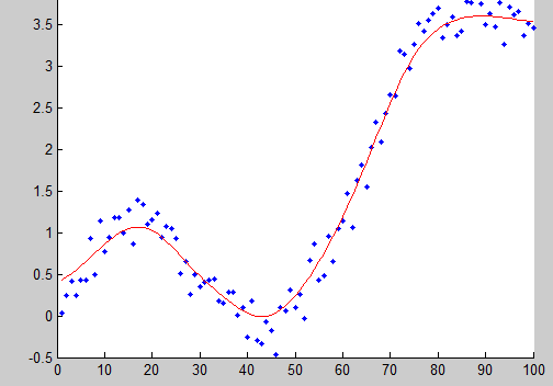
Example:例子:

4.9.2 Nearest neighbor smoother:最邻近平滑器:
The idea of the nearest neighbor smoother is the following. For each point $\vec{x}_0$, take $m$ nearest neighbors and estimate the value of $y(\vec{x}_0)$ by averaging the values of these neighbors.
Formally,
$h_{m}(\vec{x}_{0})=\left\|\vec{x}_{0}-\vec{x}_{[m]}\right\|$
, where
$\vec{x}_{[m]}$
is the $m$th closest to $\vec{x}_0$ neighbor, and:最近邻平滑器的概念如下。对于每个点$\vec{x}_0$,取$m$最近的邻居,并通过平均这些邻居的值来估计$y(\vec{x}_0)$的值。正式地,$h_{m}(\vec{x}_{0})=\left\|\vec{x}_{0}-\vec{x}_{[m]}\right\|$,其中$\vec{x}_{[m]}$是离$\vec{x}_0$最近的第$m$位,并且:
$$D(t)={\begin{cases}1/m&{\text{if }}|t|\leq 1\\0&{\text{otherwise}}\end{cases}} \tag{16}$$
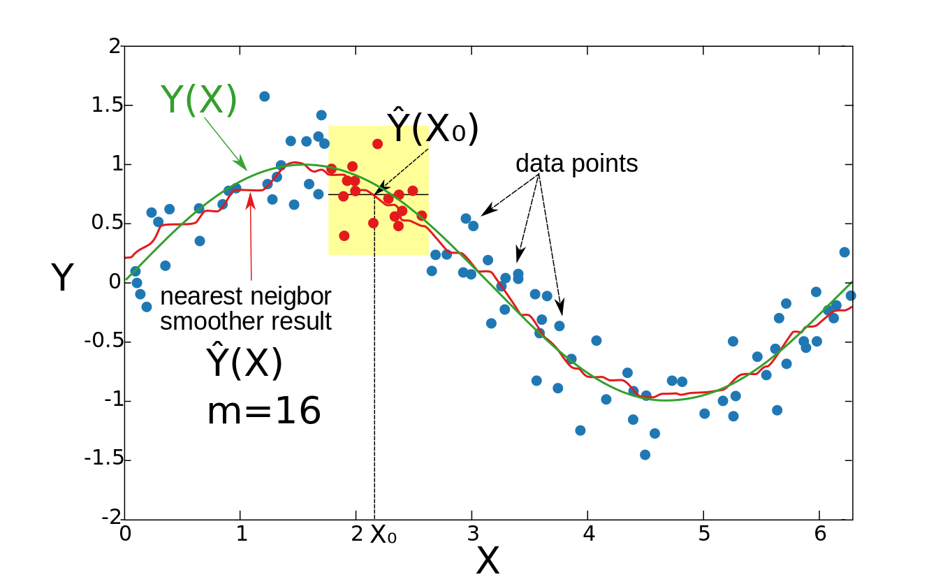
这里$t$是两点之间的距离。上式要求距离小于1是举了一个例子,并不是非得1。其实$D(t)$就是核函数,比如我们考虑取最邻近的16个点,那么就会取到核函数的16个值,代入式子(4.9.2)将求出$y(\vec{x}_0)$。
Example:例子:
 图像中标注与公式矛盾,
$X$其实该写成$\vec{x}$,$Y$其实该写成$y$,$X_0$其实该写成$\vec{x}_0$,$Y(X)$其实该写成$y(\vec{x})$,${\hat {Y}}(X)$其实该写成${\hat {y}}(\vec{x})$,${\hat {Y}}(X_0)$其实该写成${\hat {y}}(\vec{x}_0)$。后续图片相同情况。
In this example, $\vec{x}$ is one-dimensional. For each $\vec{x}_0$, the
${\hat {y}}(\vec{x}_{0})$
is an average value of 16 closest to $\vec{x}_0$ points (denoted by red). The result is not smooth enough.此例中,$\vec{x}$是一维向量(数据点、行向量)。对每个数据点$\vec{x}_0$,${\hat {y}}(\vec{x}_{0})$是16个最邻近$\vec{x}_0$的点(标记为红点)的平均的值。结果不够平滑。
4.9.3 Kernel average smoother:核平均平滑器:
The idea of the kernel average smoother is the following. For each data point $\vec{x}_0$, choose a constant distance size $\lambda$ (kernel radius, or window width for $p = 1$ dimension), and compute a weighted average for all data points that are closer than
$\lambda$
to $\vec{x}_0$ (the closer to $\vec{x}_0$ points get higher weights).
Formally,
$h_{\lambda }(\vec{x}_{0})=\lambda ={\text{constant}}$,
and $D(t)$ is one of the popular kernels.核平均平滑器的思想如下。对于每个数据点$\vec{x}_0$,选择一个固定的距离大小$\lambda$(内核半径,或$p = 1$维度的窗口宽度),并计算一个加权平均值,为所有比$\lambda$更接近$\vec{x}_0$的数据点(越接近$\vec{x}_0$的点获得更高的权重)。正式地,$h_{\lambda }(\vec{x}_{0})=\lambda ={\text{constant}}$,并且$D(t)$是最受欢迎的核之一。
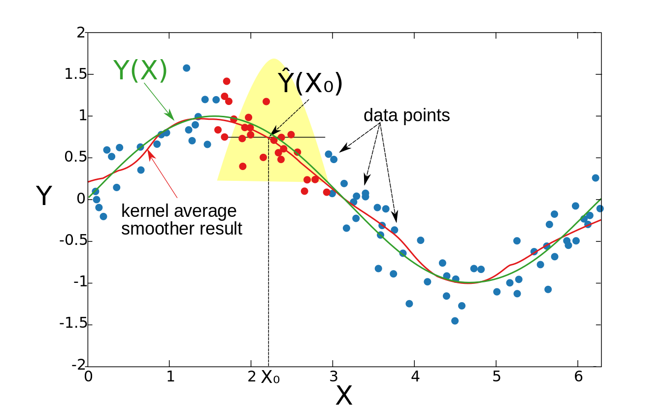
Example:例子:
 For each
 $\vec{x}_0$ the window width is constant, and the weight of each point in the window is schematically denoted by the yellow figure in the graph. It can be seen that the estimation is smooth, but the boundary points are biased. The reason for that is the non-equal number of points (from the right and from the left to the $\vec{x}_0$) in the window, when the $\vec{x}_0$ is close enough to the boundary.对每个点$\vec{x}_0$窗口宽度是常数,窗口中每个点的权重用图中黄色的图形表示。可以看出,该估计是平滑的,但边界点(这里边界点是所有$\vec{x}$的头尾)是有偏差的。原因是当$\vec{x}_0$足够接近边界时,窗口中的点(从右到$\vec{x}_0$和从左到$\vec{x}_0$)数量不相等。
4.9.4 Local linear regression:局部线性回归
In the two previous sections we assumed that the underlying $y(\vec{x})$ function is locally constant, therefore we were able to use the weighted average for the estimation. The idea of local linear regression is to fit locally a straight line (or a hyperplane for higher dimensions), and not the constant (horizontal line). After fitting the line, the estimation
${\hat {y}}(\vec{x}_{0})$
is provided by the value of this line at $\vec{x}_0$ point. By repeating this procedure for each $\vec{x}_0$, one can get the estimation function
${\hat {y}}(\vec{x})$
. Like in previous section, the window width is constant
$h_{\lambda }(\vec{x}_{0})=\lambda ={\text{constant}}$.
Formally, the local linear regression is computed by solving a weighted least square problem.在前两节(4.9.2和4.9.3)中,我们假设底层的$y(\vec{x})$函数是局部常量,因此我们可以使用加权平均值进行估计。局部线性回归的思想是在局部拟合一条直线(或高维的超平面),而不是常数(水平线)。拟合直线后,由直线在$\vec{x}_0$点处的值提供估算值${\hat {y}}(\vec{x}_{0})$。通过对每个$\vec{x}_0$重复这个过程,可以得到估计函数${\hat {y}}(\vec{x})$。与前一节(4.9.3)一样,窗体宽度是常数$h_{\lambda }(\vec{x}_{0})=\lambda ={\text{constant}}$。在形式上,局部线性回归是通过求解加权最小二乘问题来计算的。
For one dimension ($p = 1$):对一维情况($p = 1$):
$${\begin{aligned}&\min _{\alpha (\vec{x}_{0}),\beta (\vec{x}_{0})}\sum \limits _{i=1}^{N}{K_{h_{\lambda }}(\vec{x}_{0},\vec{x}_{i})\left(y(\vec{x}_{i})-\alpha (\vec{x}_{0})-\beta (\vec{x}_{0})\vec{x}_{i}\right)^{2}}\\&\,\,\,\,\,\,\,\,\,\,\,\,\,\,\,\,\,\,\,\,\,\,\,\,\,\,\,\,\,\,\,\,\,\,\,\,\,\,\,\,\,\,\,\,\,\,\,\,\,\Downarrow \\&\,\,\,\,\,\,\,\,\,\,\,\,\,\,\,\,\,\,\,\,\,\,\,\,\,{\hat {y}}(\vec{x}_{0})=\alpha (\vec{x}_{0})+\beta (\vec{x}_{0})\vec{x}_{0}\\\end{aligned}} \tag{17}$$
The closed form solution is given by:封闭形式的解由下式给出:
$${\hat {y}}(\vec{x}_{0})=\left(1,\vec{x}_{0}\right)\left(B^{T}W(\vec{x}_{0})B\right)^{-1}B^{T}W(\vec{x}_{0})y \tag{18}$$
where:其中:
$y=\left(y(\vec{x}_{1}),\dots ,y(\vec{x}_{n})\right)^{T}$$W(\vec{x}_{0})=\operatorname {diag} \left(K_{h_{\lambda }}(\vec{x}_{0},\vec{x}_{i})\right)_{n\times n}$$B^{T}=\left({\begin{matrix}1&1&\dots &1\\\vec{x}_{1}&\vec{x}_{2}&\dots &\vec{x}_{n}\\\end{matrix}}\right)$
注意到:上式是在普通线性回归中增加了局部核函数作为权值。
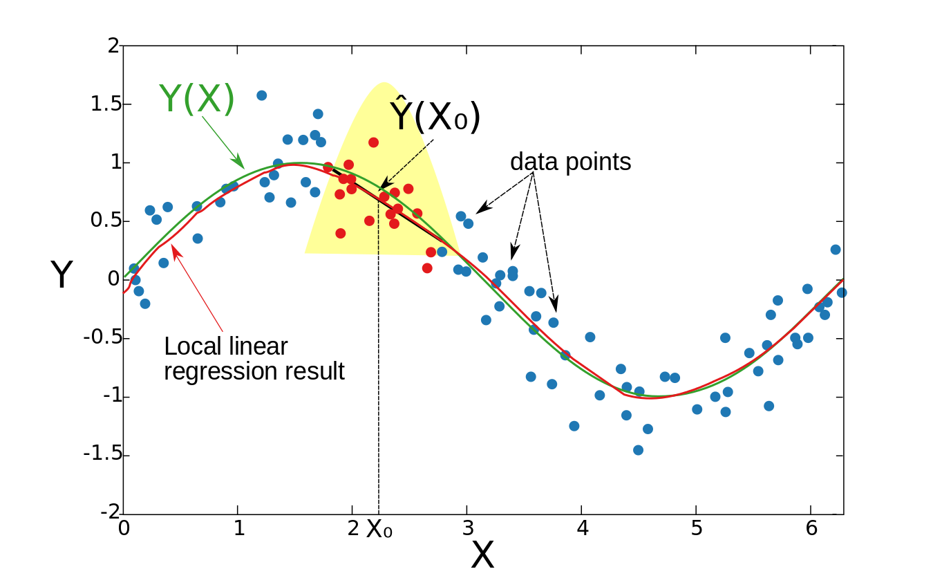
Example:例子:
 The resulting function is smooth, and the problem with the biased boundary points is solved.结果是平滑的,边界点偏差问题也不存在了。
Local linear regression can be applied to any-dimensional space, though the question of what is a local neighborhood becomes more complicated. It is common to use k nearest training points to a test point to fit the local linear regression. This can lead to high variance of the fitted function. To bound the variance, the set of training points should contain the test point in their convex hull (see Gupta et al. reference).局部线性回归可以应用于任何维空间,尽管什么是局部邻域的问题变得更加复杂。通常使用距离测试点最近的k个训练点来拟合局部线性回归。这可能导致拟合函数的方差很大。要约束方差,训练点集应该在其凸包中包含测试点(参见Gupta等人的参考文献)。
4.9.5 Local polynomial regression:局部多项式回归:
Instead of fitting locally linear functions, one can fit polynomial functions.除了拟合局部线性函数,还可以拟合多项式函数。
For $p=1$, one should minimize: 对于$p=1$,应最小化:
$${\underset {\alpha (\vec{x}_{0}),\beta _{j}(\vec{x}_{0}),j=1,...,d}{\mathop {\min } }}\,\sum \limits _{i=1}^{N}{K_{h_{\lambda }}(\vec{x}_{0},\vec{x}_{i})\left(y(\vec{x}_{i})-\alpha (\vec{x}_{0})-\sum \limits _{j=1}^{d}{\beta _{j}(\vec{x}_{0})\vec{x}_{i}^{j}}\right)^{2}} \tag{19}$$
with:有:
$${\hat {y}}(\vec{x}_{0})=\alpha (\vec{x}_{0})+\sum \limits _{j=1}^{d}{\beta _{j}(\vec{x}_{0})\vec{x}_{0}^{j}} \tag{20}$$
In general case ($p>1$), one should minimize:总体上($p>1$),应最小化:
$${\begin{aligned}&{\hat {\beta }}(\vec{x}_{0})={\underset {\beta (\vec{x}_{0})}{\mathop {\arg \min } }}\,\sum \limits _{i=1}^{N}{K_{h_{\lambda }}(\vec{x}_{0},\vec{x}_{i})\left(y(\vec{x}_{i})-b(\vec{x}_{i})^{T}\beta (\vec{x}_{0})\right)}^{2}\\&b(\vec{x})=\left({\begin{matrix}1,&\vec{x}_{1},&\vec{x}_{2},...&\vec{x}_{1}^{2},&\vec{x}_{2}^{2},...&\vec{x}_{1}\vec{x}_{2}\,\,\,...\\\end{matrix}}\right)\\&{\hat {y}}(\vec{x}_{0})=b(\vec{x}_{0})^{T}{\hat {\beta }}(\vec{x}_{0})\\\end{aligned}} \tag{21}$$
注意到:上式是在普通多项式回归中增加了局部核函数作为权值。
关于Kernel smoother的具体例子以后再掌握。有监督学习是用不上的。
参考: