集成学习ensemble_learning
The goal of ensemble methods is to combine the predictions of several base estimators built with a given learning algorithm in order to improve generalizability / robustness over a single estimator.集成方法的目标是将多个基本估计器的预测与给定的学习算法结合起来,以提高单个估计器的可通用性/鲁棒性。
Two families of ensemble methods are usually distinguished:通常分成两类不同的集成方法:
- In averaging methods, the driving principle is to build several estimators independently and then to average their predictions. On average, the combined estimator is usually better than any of the single base estimator because its variance is reduced.在平均(Averaging)方法中,驱动原理是独立构建多个估计器,然后对它们的预测进行平均(Averaging)。通过平均(Averaging),组合估计器通常优于任何单个基本估计器,因为它的方差减小了。
Examples: Bagging methods, Forests of randomized trees, …例子:装袋(Bagging)方法、随机化的森林(Forests of randomized trees)和投票分类器(Voting Classifier)等。
平均(Averaging)方法的结果集成:简单对多个基本估计器的结果进行平均(对于回归问题)、简单对多个基本估计器的结果进行多数投票(回归问题采用投票分类器的硬投票)、简单对多个基本估计器的概率结果进行平均(回归问题采用投票分类器的软投票)
- By contrast, in boosting methods, base estimators are built sequentially and one tries to reduce the bias of the combined estimator. The motivation is to combine several weak models to produce a powerful ensemble.相反,在增强(Boosting)方法中,基本估计器是按顺序建立的,并试图减少组合估计器的偏差。其动机是将几个弱模型组合成一个强大的集成。
Examples: AdaBoost, Gradient Tree Boosting, …例子:AdaBoost和梯度树增强(Gradient Tree Boosting)等。
增强(Boosting)方法的结果集成:不是简单的平均或投票,将为每个基本估计器赋予权值,这个权值本身也需要算法进行学习,然后平均或投票时候需要考虑权值。
其实还有第三种集成方法即Stacking。之后补充Stacking知识。资料见参考2,特别注意其罗列的参考资料。
1 Bagging meta-estimator装袋(Bagging)元估计器
In ensemble algorithms, bagging methods form a class of algorithms which build several instances of a black-box estimator on random subsets of the original training set and then aggregate their individual predictions to form a final prediction. These methods are used as a way to reduce the variance of a base estimator (e.g., a decision tree), by introducing randomization into its construction procedure and then making an ensemble out of it. In many cases, bagging methods constitute a very simple way to improve with respect to a single model, without making it necessary to adapt the underlying base algorithm. As they provide a way to reduce overfitting, bagging methods work best with strong and complex models (e.g., fully developed decision trees), in contrast with boosting methods which usually work best with weak models (e.g., shallow decision trees).在集成算法中,装袋(Bagging)方法形成了一类算法,这种算法在原始训练集的随机子集上构建多个黑盒估计器实例,然后将它们各自的预测集合起来形成最终的预测。这些方法通过在基本估计器(如决策树)的构造过程中引入随机化,然后对其进行集成来减少基本估计器(如决策树)的方差。在许多情况下,相对于单个模型,装袋(Bagging)方法构成了的一种非常简单的改进方法,而不需要调整底层的基本算法。由于它们提供了一种方法来减少过拟合,装袋(Bagging)方法应该运用强而复杂的模型(例如完全开发的决策树),而增强(Boosting)方法应该运用弱模型(例如浅决策树)作为基本估计器。
Bagging methods come in many flavours but mostly differ from each other by the way they draw random subsets of the training set: 装袋(Bagging)方法有很多种,但它们之间的区别主要在于它们提取训练集的随机子集的方式:
- When random subsets of the dataset are drawn as random subsets of the samples, then this algorithm is known as Pasting [B1999].当数据集的随机子集作为样本的随机子集提取时,该算法称为粘贴(Pasting)。翻译成我能懂的话:基本分类器随机抽取样本,称为粘贴(Pasting)。
- When samples are drawn with replacement, then the method is known as Bagging [B1996].当用在有放回的条件下抽取样本时,这种方法被称为装袋(Bagging)。翻译成我能懂的话:基本分类器在有放回的条件下抽取样本,称为装袋(Bagging)。
- When random subsets of the dataset are drawn as random subsets of the features, then the method is known as Random Subspaces [H1998].数据集的随机子集作为特征的随机子集提取时,该方法称为随机子空间(Random Subspaces)。翻译成我能懂的话:基本分类器随机抽取特征,称为随机子空间(Random Subspaces)。
- Finally, when base estimators are built on subsets of both samples and features, then the method is known as Random Patches [LG2012].当基估计器同时建立在样本和特征子集上时,该方法称为随机补片(Random Patches)。翻译成我能懂的话:基本估计器随机抽取样本和特征,称为随机补片(Random Patches)。
In scikit-learn, bagging methods are offered as a unified BaggingClassifier meta-estimator (resp. BaggingRegressor), taking as input a user-specified base estimator along with parameters specifying the strategy to draw random subsets. In particular, max_samples and max_features control the size of the subsets (in terms of samples and features), while bootstrap and bootstrap_features control whether samples and features are drawn with or without replacement. When using a subset of the available samples the generalization accuracy can be estimated with the out-of-bag samples by setting oob_score=True. As an example, the snippet below illustrates how to instantiate a bagging ensemble of KNeighborsClassifier base estimators, each built on random subsets of 50% of the samples and 50% of the features.在scikit-learn中,装袋(Bagging)方法作为一个统一的BaggingClassifier元估计器 (还有BaggingRegressor)提供,以用户指定的基本估计器作为输入,同时指定提取随机子集的策略参数。特别是,max_samples和max_features控制子集的大小,而bootstrap和bootstrap_features控制样本和特征的提取时是否是有放回的(bootstrap=True、bootstrap_features=True分别代表样本和特征抽样是在有放回条件下抽样)。当使用可用样本的子集时,可以通过设置oob_score=True来估计出袋(Out-Of-Bag)样本的泛化精度。作为一个例子,下面的代码片段演示了如何实例化一个由KNeighborsClassifier基本估计器组成的装袋(Bagging)集合,每个估计器都建立在50%的样本和50%的特征的随机子集上。
from sklearn.ensemble import BaggingClassifier
from sklearn.neighbors import KNeighborsClassifier
bagging = BaggingClassifier(KNeighborsClassifier(),
                            max_samples=0.5, max_features=0.5)
2 Forests of randomized trees随机树的森林
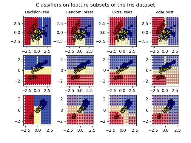
The sklearn.ensemble module includes two averaging algorithms based on randomized decision trees: the RandomForest algorithm and the Extra-Trees method. Both algorithms are perturb-and-combine techniques [B1998] specifically designed for trees. This means a diverse set of classifiers is created by introducing randomness in the classifier construction. The prediction of the ensemble is given as the averaged prediction of the individual classifiers. sklearn.ensemble模块包括两种基于随机决策树的平均(Averaging)算法:随机森林(RandomForest)算法和极端树(Extra-Trees)方法。这两种算法都是专为树设计的摄动和组合(Perturb-and-Combine)技术。这意味着通过在分类器构造中引入随机性来创建一组不同的分类器。集成预测就是单个分类器预测的平均。
As other classifiers, forest classifiers have to be fitted with two arrays: a sparse or dense array X of size [n_samples, n_features] holding the training samples, and an array Y of size [n_samples] holding the target values (class labels) for the training samples:与其他分类器一样,森林分类器需要两个数组:形状为[n_samples, n_features]的稀疏/致密数组X,用来存放训练样本;形状为[n_samples]的数组Y,用来存放训练样本的目标值(类标签)。
from sklearn.ensemble import RandomForestClassifier
X = [[0, 0], [1, 1]]
Y = [0, 1]
clf = RandomForestClassifier(n_estimators=10)
clf = clf.fit(X, Y)
Like decision trees, forests of trees also extend to multi-output problems (if Y is an array of size [n_samples, n_outputs]).和决策树一样,树的森林也可以扩展到多输出问题(如果Y是一个形状为[n_samples, n_outputs]的数组)。
2.1 Random Forests随机森林
In random forests (see RandomForestClassifier and RandomForestRegressor classes), each tree in the ensemble is built from a sample drawn with replacement (i.e., a bootstrap sample) from the training set. In addition, when splitting a node during the construction of the tree, the split that is chosen is no longer the best split among all features. Instead, the split that is picked is the best split among a random subset of the features. As a result of this randomness, the bias of the forest usually slightly increases (with respect to the bias of a single non-random tree) but, due to averaging, its variance also decreases, usually more than compensating for the increase in bias, hence yielding an overall better model.在随机森林中(参见RandomForestClassifier和RandomForestRegressor类),集成中的每棵树都是建立于在有放回的条件下提取的样本(即,一个自举(Bootstrap)样本)。此外,在树的构造过程中分割节点时,所选择的分割不再是所有特征中最好的分割。相反,所选择的分割是特征的随机子集中最好的分割。由于这种随机性,森林的偏差通常会略微增加(相对于单个非随机树的偏差而言),但由于平均(Averaging),其方差也会减少,通常方差的减少足以补偿偏差的增加,从而产生一个更好的整体模型。
In contrast to the original publication [B2001], the scikit-learn implementation combines classifiers by averaging their probabilistic prediction, instead of letting each classifier vote for a single class.与最初的发布不同,scikit-learn实现通过平均(Averaging)分类器的概率预测来组合分类器,而不是让每个分类器投票给一个类。
2.2 Extremely Randomized Trees极端随机化树
In extremely randomized trees (see ExtraTreesClassifier and ExtraTreesRegressor classes), randomness goes one step further in the way splits are computed. As in random forests, a random subset of candidate features is used, but instead of looking for the most discriminative thresholds, thresholds are drawn at random for each candidate feature and the best of these randomly-generated thresholds is picked as the splitting rule. This usually allows to reduce the variance of the model a bit more, at the expense of a slightly greater increase in bias:在极端随机化树(Extremely Randomized Trees)中(参见ExtraTreesClassifier和ExtraTreesRegressor类),在计算分割的方式上,随机性更进一步。与在随机森林中一样,使用候选特征的一个随机子集,但不是寻找最具鉴别性的阈值,而是为每个候选特征随机提取阈值,并选择这些随机生成的阈值中最佳者作为分割规则(按我理解:每个特征随机提取若干阈值,然后选择这些阈值最佳者,者意味着一个特征只划分一次。)。这通常可以使模型的方差减少一点,而代价是偏差稍微增加一点:
from sklearn.model_selection import cross_val_score
from sklearn.datasets import make_blobs
from sklearn.ensemble import RandomForestClassifier
from sklearn.ensemble import ExtraTreesClassifier
from sklearn.tree import DecisionTreeClassifier

X, y = make_blobs(n_samples=10000, n_features=10, centers=100,
    random_state=0)

clf = DecisionTreeClassifier(max_depth=None, min_samples_split=2,
    random_state=0)
scores = cross_val_score(clf, X, y, cv=5)
scores.mean()


clf = RandomForestClassifier(n_estimators=10, max_depth=None,
    min_samples_split=2, random_state=0)
scores = cross_val_score(clf, X, y, cv=5)
scores.mean()
0.999...
clf = ExtraTreesClassifier(n_estimators=10, max_depth=None,
    min_samples_split=2, random_state=0)
scores = cross_val_score(clf, X, y, cv=5)
scores.mean() > 0.999
True
2.3 Parameters参数
The main parameters to adjust when using these methods is n_estimators and max_features. The former is the number of trees in the forest. The larger the better, but also the longer it will take to compute. In addition, note that results will stop getting significantly better beyond a critical number of trees. The latter is the size of the random subsets of features to consider when splitting a node. The lower the greater the reduction of variance, but also the greater the increase in bias. Empirical good default values are max_features=n_features for regression problems, and max_features=sqrt(n_features) for classification tasks (where n_features is the number of features in the data). Good results are often achieved when setting max_depth=None in combination with min_samples_split=2 (i.e., when fully developing the trees). Bear in mind though that these values are usually not optimal, and might result in models that consume a lot of RAM. The best parameter values should always be cross-validated. In addition, note that in random forests, bootstrap samples are used by default (bootstrap=True) while the default strategy for extra-trees is to use the whole dataset (bootstrap=False). When using bootstrap sampling the generalization accuracy can be estimated on the left out or out-of-bag samples. This can be enabled by setting oob_score=True.在使用这些方法时需要调整的主要参数是n_estimators和max_features。前者是森林中树木的数量。n_estimators越大越好,但是计算时间也越长。此外,请注意,大到某个临界值后结果不会显著改善。后者是分割节点时要考虑的随机特征子集的大小。max_features越小,方差越小,偏倚越大。经验上好的默认值是用于回归问题的max_features=n_features,用于分类任务的max_features=sqrt(n_features)(其中n_features是数据中的特征数量)。设置max_depth=None并min_samples_split=2(即充分开发树)通常能达到好的结果(指很好的拟合,但很多时候已经过拟合了,所以下句说不是最优的)。请记住,这些值通常不是最优的,并且可能导致模型消耗大量RAM。最好的参数值总是应该交叉验证。此外,请注意,在随机森林(Random Forests)中,默认情况下使用自举(Bootstrap)样本(bootstrap=True),而极端树(Extra-Trees)的默认策略是使用整个数据集(bootstrap=False)。在使用自举(Bootstrap)抽样时,可以用留置样本或出袋(Out-Of-Bag)样本上估计泛化精度。这可以通过设置oob_score=True来启用(oob_score=True代表使用出袋(Out-Of-Bag)样本评估精度,否则是使用留置样本)。
- Note: The size of the model with the default parameters is
$O( M * N * log (N) )$, where$M$is the number of trees and$N$is the number of samples. In order to reduce the size of the model, you can change these parameters:min_samples_split,max_leaf_nodes,max_depthandmin_samples_leaf.注:默认参数下模型大小为$O( M * N * log (N) )$,其中$M$是树的数目$N$是样本数。为了减小模型的大小,可以更改这些参数:min_samples_split、max_leaf_nodes、max_depth和min_samples_leaf。
2.4 Parallelization并行化
Finally, this module also features the parallel construction of the trees and the parallel computation of the predictions through the n_jobs parameter. If n_jobs=k then computations are partitioned into k jobs, and run on k cores of the machine. If n_jobs=-1 then all cores available on the machine are used. Note that because of inter-process communication overhead, the speedup might not be linear (i.e., using k jobs will unfortunately not be k times as fast). Significant speedup can still be achieved though when building a large number of trees, or when building a single tree requires a fair amount of time (e.g., on large datasets).最后,该模块还具有树的并行构造和通过n_jobs参数进行预测的并行计算。如果n_jobs=k,则计算被划分为k个工作,并在机器的k个核心上运行。如果n_jobs=-1,则使用机器上可用的所有核心。注意,由于进程间通信开销,加速可能不是线性的(也就是,不幸的是,使用k个工作的速度不会快上k倍)。但是,当构建大量的树或构建单个树需要相当长的时间(例如,在大型数据集中)时,仍然可以实现显著地加速。
2.5 Feature importance evaluation特征重要度计算
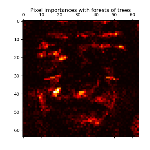
The relative rank (i.e. depth) of a feature used as a decision node in a tree can be used to assess the relative importance of that feature with respect to the predictability of the target variable. Features used at the top of the tree contribute to the final prediction decision of a larger fraction of the input samples. The expected fraction of the samples they contribute to can thus be used as an estimate of the relative importance of the features. In scikit-learn, the fraction of samples a feature contributes to is combined with the decrease in impurity from splitting them to create a normalized estimate of the predictive power of that feature.作为树中决策节点的特征的相对秩(即深度)可以用来评估该特征相对于目标变量的可预测性的相对重要性。用在树顶部的特征将贡献输入样本的最大划分给最终预测决策。因此,特征贡献的期望的样本划分可以用来估计特征的相对重要性。在scikit-learn中,一个特征所贡献的样本的划分与分离时不纯度的减少相结合,从而对该特征的预测能力进行评估,特征重要性将规范化使和为1。
By averaging the estimates of predictive ability over several randomized trees one can reduce the variance of such an estimate and use it for feature selection. This is known as the mean decrease in impurity, or MDI. Refer to [L2014] for more information on MDI and feature importance evaluation with Random Forests.通过对几个随机树的预测能力的估计进行平均(Averaging),可以减少这种估计的方差,并将其用于特征选择。这被称为不纯度的平均减少(Mean Decrease in Impurity),或MDI。
 In practice those estimates are stored as an attribute named
 feature_importances_ on the fitted model. This is an array with shape (n_features,) whose values are positive and sum to 1.0. The higher the value, the more important is the contribution of the matching feature to the prediction function.在实践中,这些估算值作为一个名为feature_importances_的属性存储在拟合模型中。这是一个具有形状(n_features,)的数组,其值为正数,和为1.0。值越大,相应特征对预测函数的贡献越大。
2.6 Totally Random Trees Embedding完全随机树嵌入
RandomTreesEmbedding implements an unsupervised transformation of the data. Using a forest of completely random trees, RandomTreesEmbedding encodes the data by the indices of the leaves a data point ends up in. This index is then encoded in a one-of-K manner, leading to a high dimensional, sparse binary coding. This coding can be computed very efficiently and can then be used as a basis for other learning tasks. The size and sparsity of the code can be influenced by choosing the number of trees and the maximum depth per tree. For each tree in the ensemble, the coding contains one entry of one. The size of the coding is at most n_estimators * 2 ** max_depth, the maximum number of leaves in the forest. RandomTreesEmbedding实现了数据的无监督转换。使用完全随机的树组成的森林,RandomTreesEmbedding通过数据点最终所在的叶子的索引对数据进行编码。然后这个索引以k列独热方式编码,从而得到一个高维的稀疏二值编码。这种编码可以非常有效地计算,然后可以作为其他学习任务的基础。可以通过选择树的数量和每棵树的最大深度来影响编码的大小和稀疏性。对于集成中的每一棵树,编码都包含其中的一个条目。编码的大小最多是n_estimators * 2 ** max_depth,即森林中叶子的最大数量。
无监督学习不存在目标变量,那么根据什么不纯度(Impurity)来划分数据?查阅sklearn文档之sklearn.ensemble.RandomTreesEmbedding函数仍未能找到答案。既然不影响后续理解,那先放下吧。
As neighboring data points are more likely to lie within the same leaf of a tree, the transformation performs an implicit, non-parametric density estimation.由于相邻的数据点更有可能位于树的同一叶片内,因此该转换执行隐式的非参数密度估计。
3 AdaBoost
The module sklearn.ensemble includes the popular boosting algorithm AdaBoost, introduced in 1995 by Freund and Schapire [FS1995].模块sklearn.ensemble包括流行的增强(Boosting)算法AdaBoost,由Freund和Schapire于1995年引入。
The core principle of AdaBoost is to fit a sequence of weak learners (i.e., models that are only slightly better than random guessing, such as small decision trees) on repeatedly modified versions of the data. The predictions from all of them are then combined through a weighted majority vote (or sum) to produce the final prediction. The data modifications at each so-called boosting iteration consist of applying weights
$w_1,w_2,\ldots, w_n$
to each of the training samples. Initially, those weights are all set to
$w_i = 1/N$
, so that the first step simply trains a weak learner on the original data. For each successive iteration, the sample weights are individually modified and the learning algorithm is reapplied to the reweighted data. At a given step, those training examples that were incorrectly predicted by the boosted model induced at the previous step have their weights increased, whereas the weights are decreased for those that were predicted correctly. As iterations proceed, examples that are difficult to predict receive ever-increasing influence. Each subsequent weak learner is thereby forced to concentrate on the examples that are missed by the previous ones in the sequence [HTF]. AdaBoost的核心原则是用一序列的弱学习器(即在重复修改的数据版本上,只比随机猜测稍好一点的模型,比如小的决策树),每个学习器重复对数据集修改并训练。所有学习器预测的加权多数投票(或加权合计)产生最终预测。每个所谓的增强(Boosting)迭代的数据修改包括对每个训练样本应用权重$w_1,w_2,\ldots, w_n$。最初,这些权重都被设置为$w_i = 1/N$,因此第一步只是在原始数据上训练弱学习器。对于接下来的迭代,分别修改样本权值,并将学习算法重新应用到新权值的数据上。在给定的步骤中,用前一步诱导增强后的(Boosted)模型进行预测,预测错误的训练样本其权重会增加,而预测正确的训练样本的权重会减少。随着迭代的进行,很难预测的样本(的权重)会受到越来越大的影响。因此,随后的每一个弱学习器都被迫将注意力集中在序列中先前的弱学习器失误的例子上。
 AdaBoost can be used both for classification and regression problems: AdaBoost可同时用于分类和回归问题:
- For multi-class classification,
AdaBoostClassifierimplements AdaBoost-SAMME and AdaBoost-SAMME.R [ZZRH2009].对多分类,AdaBoostClassifier应用AdaBoost-SAMME和AdaBoost-SAMME.R。 - For regression,
AdaBoostRegressorimplements AdaBoost.R2 [D1997].对回归,AdaBoostRegressor应用AdaBoost.R2。
AdaBoostClassifier函数有参数algorithm可选‘SAMME’、‘SAMME.R’,而AdaBoostRegressor目前仅能使用AdaBoost.R2算法。这三个算法应该是关于权重如何初始并迭代的算法。
AdaBoost并不要求基本估计器必须是决策树,任何支持样本行权(Sample Weighting)的估计器均可,;这点上与GBRT是不同的,GBRT的基本估计器必须是某种决策树(按名字是某种回归树?),我们仅能通过max_depth等设置树的形状。
AdaBoost的以上介绍还留有如下疑问:AdaBoost使用何种结果集成策略?或者应该新开一博文专门介绍,刘建平Pinard-集成学习之Adaboost算法原理小结 是一篇很好的介绍博文。
3.1 Usage使用
The following example shows how to fit an AdaBoost classifier with 100 weak learners:下例示意用100个弱学习器训练AdaBoost分类器:
from sklearn.model_selection import cross_val_score
from sklearn.datasets import load_iris
from sklearn.ensemble import AdaBoostClassifier

iris = load_iris()
clf = AdaBoostClassifier(n_estimators=100)
scores = cross_val_score(clf, iris.data, iris.target, cv=5)
scores.mean()
0.9...
The number of weak learners is controlled by the parameter n_estimators. The learning_rate parameter controls the contribution of the weak learners in the final combination. By default, weak learners are decision stumps. Different weak learners can be specified through the base_estimator parameter. The main parameters to tune to obtain good results are n_estimators and the complexity of the base estimators (e.g., its depth max_depth or minimum required number of samples to consider a split min_samples_split).弱学习器的数量由参数n_estimators控制。learning_rate参数控制弱学习器在最终组合中的贡献。默认情况下,弱学习器是决策树桩(也就是深度为1的树,base_estimator=DecisionTreeClassifier(max_depth=1))。可以通过base_estimator参数指定不同的弱学习器。为了获得好的结果,需要进行优化的主要参数是n_estimators和基本估计器的复杂度(例如,它的深度max_depth或考虑拆分所需的最小样本数量min_samples_split)。
4 Gradient Tree Boosting梯度树增强
Gradient Tree Boosting or Gradient Boosted Regression Trees (GBRT) is a generalization of boosting to arbitrary differentiable loss functions. GBRT is an accurate and effective off-the-shelf procedure that can be used for both regression and classification problems.梯度树增强(Gradient Tree Boosting)或梯度增强回归树(Gradient Boosted Regression Trees)(GBRT)是对任意可微损失函数增强(Boosting)推广。GBRT是一种精确有效的现成程序,可用于回归问题和分类问题。
GBDT(Gradient Boosting Decison Trees)=GBRT(Gradient Boosted Regression Trees/Gradient Boosting Regression Trees)=GBT(Gradient Boosting Trees)=GTB(Gradient Trees Boosting)=MART(Multiple Additive Regression Trees)一个意思。
Gradient Tree Boosting models are used in a variety of areas including Web search ranking and ecology.梯度树增强(Gradient Tree Boosting)模型应用于各种领域,包括网络搜索排名和生态系统。
The advantages of GBRT are: GBRT之优势:
- Natural handling of data of mixed type (= heterogeneous features)混合类型数据的自然处理(即多样化特征)
- Predictive power预测能力(相对于SVM)
- Robustness to outliers in output space (via robust loss functions)对输出空间中离群值的鲁棒性(通过鲁棒损失函数)
The disadvantages of GBRT are: GBRT之劣势:
- Scalability, due to the sequential nature of boosting it can hardly be parallelized.扩展性,由于增强(Boosting)的顺序性,它很难并行化。
The module sklearn.ensemble provides methods for both classification and regression via gradient boosted regression trees.模块sklearn.ensemble提供了通过梯度增强回归树(Gradient Boosted Regression Trees)进行分类和回归的方法。
4.1 Classification分类
GradientBoostingClassifier supports both binary and multi-class classification. The following example shows how to fit a gradient boosting classifier with 100 decision stumps as weak learners: GradientBoostingClassifier支持二分类和多类分类。下面的例子展示了如何训练由100个决策树桩作为弱学习器构成的一个梯度增强(Gradient Boosting)分类器:
from sklearn.datasets import make_hastie_10_2
from sklearn.ensemble import GradientBoostingClassifier

X, y = make_hastie_10_2(random_state=0)
X_train, X_test = X[:2000], X[2000:]
y_train, y_test = y[:2000], y[2000:]

clf = GradientBoostingClassifier(n_estimators=100, learning_rate=1.0,
    max_depth=1, random_state=0).fit(X_train, y_train)
clf.score(X_test, y_test)
0.913...
The number of weak learners (i.e. regression trees) is controlled by the parameter n_estimators; The size of each tree can be controlled either by setting the tree depth via max_depth or by setting the number of leaf nodes via max_leaf_nodes. The learning_rate is a hyper-parameter in the range (0.0, 1.0] that controls overfitting via shrinkage .弱学习器的数量(即回归树)由参数n_estimators控制;每棵树的大小可以通过max_depth来设置树的深度,也可以通过max_leaf_nodes来设置叶节点的数量来控制。learning_rate是范围为(0.0, 1.0]的超参,收缩(Shrinkage)其值可防止过拟合。
- Note: Classification with more than 2 classes requires the induction of
n_classesregression trees at each iteration, thus, the total number of induced trees equalsn_classes * n_estimators. For datasets with a large number of classes we strongly recommend to useRandomForestClassifieras an alternative toGradientBoostingClassifier.注:2类以上的分类需要在每次迭代中归纳出n_classes回归树,因此归纳出的树的总数等于n_classes * n_estimators。对于具有大量类的数据集,强烈建议使用RandomForestClassifier作为GradientBoostingClassifier的替代方法。
4.2 Regression回归
GradientBoostingRegressor supports a number of different loss functions for regression which can be specified via the argument loss; the default loss function for regression is least squares ('ls').GradientBoostingRegressor支持许多不同的损失函数,可以通过参数loss来指定;回归的默认损失函数是最小二乘('ls')。
import numpy as np
from sklearn.metrics import mean_squared_error
from sklearn.datasets import make_friedman1
from sklearn.ensemble import GradientBoostingRegressor

X, y = make_friedman1(n_samples=1200, random_state=0, noise=1.0)
X_train, X_test = X[:200], X[200:]
y_train, y_test = y[:200], y[200:]
est = GradientBoostingRegressor(n_estimators=100, learning_rate=0.1,
    max_depth=1, random_state=0, loss='ls').fit(X_train, y_train)
mean_squared_error(y_test, est.predict(X_test))
5.00...
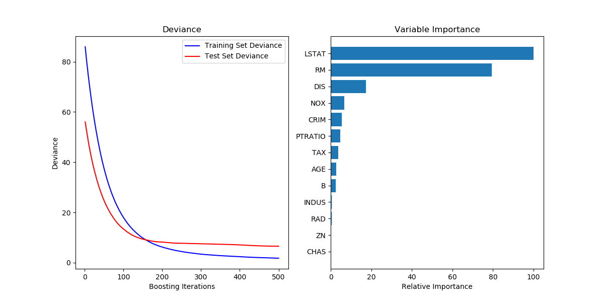
The figure below shows the results of applying GradientBoostingRegressor with least squares loss and 500 base learners to the Boston house price dataset (sklearn.datasets.load_boston). The plot on the left shows the train and test error at each iteration. The train error at each iteration is stored in the train_score_ attribute of the gradient boosting model. The test error at each iterations can be obtained via the staged_predict method which returns a generator that yields the predictions at each stage. Plots like these can be used to determine the optimal number of trees (i.e. n_estimators) by early stopping. The plot on the right shows the feature importances which can be obtained via the feature_importances_ property.下图显示了在波士顿房价数据集(sklearn.datasets.load_boston)中应用GradientBoostingRegressor(最小二乘损失、500个基本学习器)的结果。左边的图显示了每次迭代的训练和测试误差。每次迭代训练误差储存在梯度增强(gradient boosting)模型的train_score_属性值中。每次迭代测试误差可以通staged_predict方法得到,该方法返回一个生成器,生成每个阶段的预测。像这样的图可以用来确定树的最优数量,之后可设置n_estimators来实现树的最优数量。
4.3 Fitting additional weak-learners训练附加弱学习器
Both GradientBoostingRegressor and GradientBoostingClassifier support warm_start=True which allows you to add more estimators to an already fitted model. GradientBoostingRegressor和GradientBoostingClassifier都支持warm_start=True,这允许向已经拟合的模型添加更多的估计器。
_ = est.set_params(n_estimators=200, warm_start=True)  # set warm_start and new nr of trees
_ = est.fit(X_train, y_train) # fit additional 100 trees to est
mean_squared_error(y_test, est.predict(X_test))
3.84...
4.4 Controlling the tree size控制树大小
The size of the regression tree base learners defines the level of variable interactions that can be captured by the gradient boosting model. In general, a tree of depth h can capture interactions of order h . There are two ways in which the size of the individual regression trees can be controlled.回归树(Regression Tree)基本学习器的大小定义了梯度增强(Gradient Boosting)模型可以捕获的变量交互的级别。一般来说,深度h的树可以捕捉到顺序h的相互作用。有两种方法可以控制单个回归树的大小。
If you specify max_depth=h then complete binary trees of depth h will be grown. Such trees will have (at most) 2**h leaf nodes and 2**h - 1 split nodes.如果指定max_depth=h,则将生成深度为h的完整二叉树。这些树最多有2**h叶节点和2**h - 1分裂节点。
Alternatively, you can control the tree size by specifying the number of leaf nodes via the parameter max_leaf_nodes. In this case, trees will be grown using best-first search where nodes with the highest improvement in impurity will be expanded first. A tree with max_leaf_nodes=k has k - 1 split nodes and thus can model interactions of up to order max_leaf_nodes - 1 .或者,您可以通过参数max_leaf_nodes指定叶子节点的数量来控制树的大小。在这种情况下,将使用最好的优先策略进行搜索,不纯度改善程度最高的节点将优先扩展。max_leaf_nodes=k的树具有k - 1分裂节点,因此可以对高达max_leaf_nodes - 1的交互排序进行建模。
We found that max_leaf_nodes=k gives comparable results to max_depth=k-1 but is significantly faster to train at the expense of a slightly higher training error. The parameter max_leaf_nodes corresponds to the variable J in the chapter on gradient boosting in [F2001] and is related to the parameter interaction.depth in R’s gbm package where max_leaf_nodes == interaction.depth + 1 .我们发现,max_leaf_nodes=k的结果与max_depth=k-1相当,但训练速度要快得多,代价是训练误差略高。
4.5 Mathematical formulation数学公式
GBRT considers additive models of the following form:GBRT考虑以下形式的加法模型:
$$F(x) = \sum_{m=1}^{M} \gamma_m h_m(x) \tag{1}$$
$h_m(x)$是第$m$个基本估计器,$M$是基本估计器的数量即n_estimators,$F(x)$是全部$M$个基本估计器集成后的估计器,最终预测就是根据这个集成估计器。
where
$h_m(x)$
are the basis functions which are usually called weak learners in the context of boosting. Gradient Tree Boosting uses decision trees of fixed size as weak learners. Decision trees have a number of abilities that make them valuable for boosting, namely the ability to handle data of mixed type and the ability to model complex functions.其中$h_m(x)$是基本函数,在增强(Boosting)语境中通常称为弱学习器。梯度树增强(Gradient Tree Boosting)使用固定大小的决策树作为弱学习器。决策树具有多种能力,这些能力使其具有增强(Boosting)的价值,即处理混合类型数据的能力和对复杂函数建模的能力。
Similar to other boosting algorithms, GBRT builds the additive model in a greedy fashion:类似其他增强(Boosting)算法,GBRT以贪婪的方式构建加法模型:
$$F_m(x) = F_{m-1}(x) + \gamma_m h_m(x) \tag{2}$$
$F_m(x)$是前$m$个基本估计器组成的集成后的估计器,$h_m(x)$是第$m$个基本估计器,$F_{m-1}(x)$是前$m-1$个基本估计器组成的集成后的估计器。
where the newly added tree
$h_m$
tries to minimize the loss
$L$
, given the previous ensemble
$F_{m-1}$
:给定之前的集合$F_{m-1}$,新添加的树$h_m$试图最小化损失$L$:
$$h_m =  \arg\min_{h} \sum_{i=1}^{n} L\left(y_i,
F_{m-1}(x_i) + \gamma_m h(x_i)\right) \tag{3}$$
将(2)式代入损失函数并最小化损失函数本来可以同时求$h_m$和$\gamma_m$,即二者的联合最优。但GBRT不需要二者的联合最优,其假设$h_m$是$F_{m-1}$的负梯度,如(5)式所示。根据负梯度假设,在根据(6)式可以求出$\gamma_m$。将$\gamma_m$代入上式即可求出$h_m$。
也可根据(5)式求出$h_m$,最小化损失求出$h_m$。
The initial model
$F_{0}$
is problem specific, for least-squares regression one usually chooses the mean of the target values.初始模型$F_{0}$是随问题不同而不同的,对于最小二乘回归,通常选择目标值的均值。
- Note: The initial model can also be specified via the
initargument. The passed object has to implementfitandpredict.注:初始模型也可以通过init参数指定。传递的对象必须应用fit和predict。
Gradient Boosting attempts to solve this minimization problem numerically via steepest descent: The steepest descent direction is the negative gradient of the loss function evaluated at the current model
$F_{m-1}$
which can be calculated for any differentiable loss function:梯度增强法(Gradient Boosting)试图通过最速下降法数值化求解这一极小化问题:最速下降方向是在当前模型$F_{m-1}$下计算的损失函数的负梯度,可以对任何可微损失函数进行计算:
$$F_m(x) = F_{m-1}(x) - \gamma_m \sum_{i=1}^{n} \nabla_F L\left(y_i,
F_{m-1}(x_i)\right) \tag{4}$$
(4)式与(2)式比较发现$$h_m(x) = -\sum_{i=1}^{n} \nabla_F L\left(y_i,
F_{m-1}(x_i)\right) \tag{5}$$。
Where the step length
$\gamma_m$
is chosen using line search:其中步长$\gamma_m$根据线性搜索:
$$\gamma_m = \arg\min_{\gamma} \sum_{i=1}^{n} L\left(y_i, F_{m-1}(x_i)
- \gamma \frac{\partial L(y_i, F_{m-1}(x_i))}{\partial F_{m-1}(x_i)}\right) \tag{6}$$
(6)式其实就是将(4)式代入损失函数,最小化损失以求得$\gamma_m$。
根据$if \ h \in \mathcal{H}, \ then \ \gamma h \in \mathcal{H} \text{ for all } h \in \mathbb{R}$,所以可直接令$\gamma_1=1$,而不用根据(6)式求$\gamma_1$,而且根据(6)式也求不出$\gamma_1$。
The algorithms for regression and classification only differ in the concrete loss function used.回归和分类的算法只是在具体的损失函数使用上有所不同。
4.5.1 Loss Functions损失函数
The following loss functions are supported and can be specified using the parameter loss:支持以下损失函数,可以使用参数loss指定:
- Regression回归
- Least squares (
'ls'): The natural choice for regression due to its superior computational properties. The initial model is given by the mean of the target values.最小二乘('ls'):回归的自然选择,由于其优越的计算性能。初始模型由目标值的均值给出。 - Least absolute deviation (
'lad'): A robust loss function for regression. The initial model is given by the median of the target values.最小绝对偏差('lad'):用于回归的鲁棒损失函数。初始模型由目标值的中值给出。 - Huber (
'huber'): Another robust loss function that combines least squares and least absolute deviation; usealphato control the sensitivity with regards to outliers (see [F2001] for more details). Huber('huber'):另一种鲁棒损失函数,其是最小二乘和最小绝对偏差的联合;使用alpha来控制对异常值的敏感性。 - Quantile (
'quantile'): A loss function for quantile regression. Use0 < alpha < 1to specify the quantile. This loss function can be used to create prediction intervals (see Prediction Intervals for Gradient Boosting Regression). 分位数('quantile'):分位数回归的损失函数。使用0 < alpha < 1来设置分位数。这个损失函数可以用来创建预测值的区间。
- Least squares (
- Classification分类
- Binomial deviance (
'deviance'): The negative binomial log-likelihood loss function for binary classification (provides probability estimates). The initial model is given by the log odds-ratio.二项式偏差('deviance'):二值分类的负二项对数似然损失函数(提供概率估计)。初始模型由对数优势比给出。 - Multinomial deviance (
'deviance'): The negative multinomial log-likelihood loss function for multi-class classification withn_classesmutually exclusive classes. It provides probability estimates. The initial model is given by the prior probability of each class. At each iterationn_classesregression trees have to be constructed which makes GBRT rather inefficient for data sets with a large number of classes.多项式偏差('deviance'):具有n_classes互斥分类的多分类的负多项式对数似然损失函数。提供概率估计。初始模型由每个类的先验概率给出。在每次迭代中,必须构造n_classes回归树,这使得GBRT对于具有大量类的数据集来说相当低效。 - Exponential loss (
'exponential'): The same loss function asAdaBoostClassifier. Less robust to mislabeled examples than'deviance'; can only be used for binary classification.指数损失('exponential'):与AdaBoostClassifier相同的损失函数。对于错误标签的例子,不如'deviance'那么鲁棒;只能用于二值分类。
- Binomial deviance (
4.6 Regularization正则化
4.6.1 Shrinkage收缩
[F2001] proposed a simple regularization strategy that scales the contribution of each weak learner by a factor
$\nu$
:[F2001]提出了一种简单的正则化策略,该策略通过一个因子$\nu$来衡量每个弱学习器的贡献:
$$F_m(x) = F_{m-1}(x) + \nu \gamma_m h_m(x) \tag{7}$$
学习率是高参,只能网格搜索获得最优,不能被学习器本身学得。
The parameter
$\nu$
is also called the learning rate because it scales the step length the gradient descent procedure; it can be set via the learning_rate parameter.参数$\nu$也被称为学习率,因为它缩放了步长和梯度下降过程;可以通过learning_rate参数进行设置。
The parameter learning_rate strongly interacts with the parameter n_estimators, the number of weak learners to fit. Smaller values of learning_rate require larger numbers of weak learners to maintain a constant training error. Empirical evidence suggests that small values of learning_rate favor better test error. [HTF2009] recommend to set the learning rate to a small constant (e.g. learning_rate <= 0.1) and choose n_estimators by early stopping. For a more detailed discussion of the interaction between learning_rate and n_estimators see [R2007].参数learning_rate与参数n_estimators(要训练的弱学习器数量)强烈交互。learning_rate的值越小,就需要更多的弱学习器来维持常数训练误差。[HTF2009]建议将学习率设置为一个小常数(例如learning_rate <= 0.1),通过提前停止选择n_estimators。
4.6.2 Subsampling子抽样
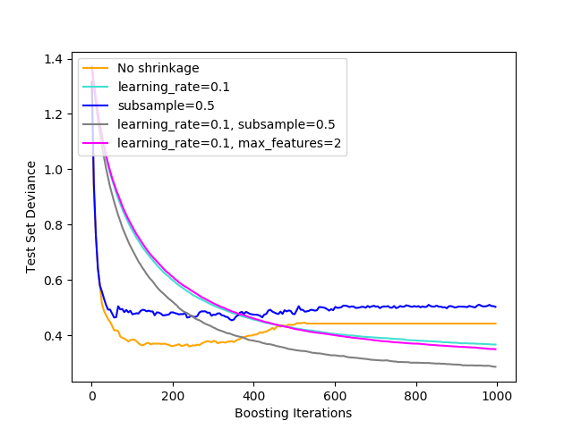
[F1999] proposed stochastic gradient boosting, which combines gradient boosting with bootstrap averaging (bagging). At each iteration the base classifier is trained on a fraction subsample of the available training data. The subsample is drawn without replacement. A typical value of subsample is 0.5. [F1999]提出了将梯度增强(Gradient Boosting)与自举(Bootstrap)平均(Averaging)(装袋(Bagging))相结合的随机梯度增强方法。在每次迭代中,基本分类器都是在可用训练数据的一小部分subsample上训练的。subsample是在无放回的条件下提取出来的。subsample的典型值是0.5。
The figure below illustrates the effect of shrinkage and subsampling on the goodness-of-fit of the model. We can clearly see that shrinkage outperforms no-shrinkage. Subsampling with shrinkage can further increase the accuracy of the model. Subsampling without shrinkage, on the other hand, does poorly.下图说明了收缩(Shrinkage)和子抽样(Subsampling)对模型拟合优度的影响。我们可以清楚地看到,收缩优于无收缩(Shrinkage)。带收缩(Shrinkage)的子抽样(Subsampling)可以进一步提高模型的精度。另一方面,没有收缩(Shrinkage)的子抽样(Subsampling)效果很差。
 Another strategy to reduce the variance is by subsampling the features analogous to the random splits in
 RandomForestClassifier. The number of subsampled features can be controlled via the max_features parameter.另一种减少方差的策略是对特征进行子抽样(Subsampling),类似于RandomForestClassifier中的随机分割。子采样后的特征的数量可以通过max_features参数来控制。
- Note: Using a small
max_featuresvalue can significantly decrease the runtime.注:使用一个小的max_features值可以显著减少运行时间。
Stochastic gradient boosting allows to compute out-of-bag estimates of the test deviance by computing the improvement in deviance on the examples that are not included in the bootstrap sample (i.e. the out-of-bag examples). The improvements are stored in the attribute oob_improvement_. oob_improvement_[i] holds the improvement in terms of the loss on the OOB samples if you add the i-th stage to the current predictions. Out-of-bag estimates can be used for model selection, for example to determine the optimal number of iterations. OOB estimates are usually very pessimistic thus we recommend to use cross-validation instead and only use OOB if cross-validation is too time consuming.随机梯度增强(Stochastic Gradient Boosting)允许通过计算未包含在自举(Bootstrap)样本(即出袋(Out-Of-Bag)样本)中的样本的偏差改进来计算测试偏差的出袋(Out-Of-Bag)估计。改进存储在属性oob_improvement_中。oob_improvement_[i]是指如果将第i阶段添加到当前预测中,就OOB样本的损失而言的改进。出袋(Out-Of-Bag)估计可以用于模型选择,例如确定最优的迭代次数。OOB估计通常非常悲观,因此我们建议使用交叉验证,只有在交叉验证太耗时时才使用OOB。
4.7 Interpretation解释
Individual decision trees can be interpreted easily by simply visualizing the tree structure. Gradient boosting models, however, comprise hundreds of regression trees thus they cannot be easily interpreted by visual inspection of the individual trees. Fortunately, a number of techniques have been proposed to summarize and interpret gradient boosting models.单个决策树可以简单地通过可视化树结构来解释。然而,梯度增强(Gradient Boosting)模型包含数百个回归树,因此它们不能通过对单个树的可视化检查轻易地解释。幸运的是,已经提出了许多技术来总结和解释梯度增强(Gradient Boosting)模型。
4.7.1 Feature importance特征重要度
Often features do not contribute equally to predict the target response; in many situations the majority of the features are in fact irrelevant. When interpreting a model, the first question usually is: what are those important features and how do they contributing in predicting the target response?通常特征对预测目标响应的贡献并不相等;在许多情况下,大多数特征实际上是不相关的。在解释模型时,第一个问题通常是:重要的特征是那些?它们在预测目标响应方面有什么贡献?
Individual decision trees intrinsically perform feature selection by selecting appropriate split points. This information can be used to measure the importance of each feature; the basic idea is: the more often a feature is used in the split points of a tree the more important that feature is. This notion of importance can be extended to decision tree ensembles by simply averaging the feature importance of each tree (see Feature importance evaluation for more details).单个决策树通过选择合适的分割点本质上执行特征选择。这些信息可以用来衡量每个特征的重要性;基本思想是:在树的分叉点上使用一个特征的频率越高,这个特征就越重要。通过简单地平均(Averaging)每棵树的特征重要性,这个重要性的概念可以扩展到决策树集合(更多细节请参见特征重要性评估)。
The feature importance scores of a fit gradient boosting model can be accessed via the feature_importances_ property:通过feature_importances_属性,可以获取梯度增强(Gradient Boosting)模型的特征重要度得分:
from sklearn.datasets import make_hastie_10_2
from sklearn.ensemble import GradientBoostingClassifier

X, y = make_hastie_10_2(random_state=0)
clf = GradientBoostingClassifier(n_estimators=100, learning_rate=1.0,
    max_depth=1, random_state=0).fit(X, y)
clf.feature_importances_
array([0.10..., 0.10..., 0.11..., ...
4.7.2 Partial dependence部分依赖
Partial dependence plots (PDP) show the dependence between the target response and a set of ‘target’ features, marginalizing over the values of all other features (the ‘complement’ features). Intuitively, we can interpret the partial dependence as the expected target response [1] as a function of the ‘target’ features [2].部分依赖图(PDP)显示了目标响应和一组目标特征之间的依赖关系,忽略了所有其他特征(补充特征)的值。直观上,我们可以将部分依赖关系解释为预期目标响应作为目标特征的函数。
Due to the limits of human perception the size of the target feature set must be small (usually, one or two) thus the target features are usually chosen among the most important features.由于人类感知的限制,目标特征集的大小必须很小(通常是一个或两个),因此目标特征通常是最重要的特征之一。
The Figure below shows four one-way and one two-way partial dependence plots for the California housing dataset:下图显示了加利福尼亚住房数据集的四个单向和一个双向部分依赖关系图:
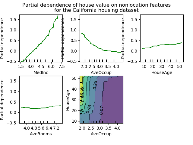 One-way PDPs tell us about the interaction between the target response and the target feature (e.g. linear, non-linear). The upper left plot in the above Figure shows the effect of the median income in a district on the median house price; we can clearly see a linear relationship among them.单向PDP告诉我们目标响应和目标特征之间的相互作用(例如线性、非线性)。上图左上方的图显示了一个地区的收入中位数对房价中位数的影响;我们可以清楚地看到它们之间的线性关系。
PDPs with two target features show the interactions among the two features. For example, the two-variable PDP in the above Figure shows the dependence of median house price on joint values of house age and avg. occupants per household. We can clearly see an interaction between the two features: For an avg. occupancy greater than two, the house price is nearly independent of the house age, whereas for values less than two there is a strong dependence on age.带有两个目标特征的PDP显示了这两个特征之间的交互作用。例如,上图中的双变量PDP显示了房价中值对每户居民房屋年龄和平均房价联合值的依赖关系。我们可以清楚地看到这两个特征之间的相互作用:当平均入住率大于2时,房价几乎与房屋年龄无关,而当平均入住率小于2时,则与年龄有很强的相关性。
The module partial_dependence provides a convenience function plot_partial_dependence to create one-way and two-way partial dependence plots. In the below example we show how to create a grid of partial dependence plots: two one-way PDPs for the features 0 and 1 and a two-way PDP between the two features:模块partial_dependence提供了方便的函数plot_partial_dependence,来创建单向和双向部分依赖关系图。在下面的样本中,我们将展示如何创建一个部分依赖图网格:两个单向PDP用于特征0和1,以及两个特征之间的双向PDP:
from sklearn.datasets import make_hastie_10_2
from sklearn.ensemble import GradientBoostingClassifier
from sklearn.ensemble.partial_dependence import plot_partial_dependence

X, y = make_hastie_10_2(random_state=0)
clf = GradientBoostingClassifier(n_estimators=100, learning_rate=1.0,
    max_depth=1, random_state=0).fit(X, y)
features = [0, 1, (0, 1)]
fig, axs = plot_partial_dependence(clf, X, features)
For multi-class models, you need to set the class label for which the PDPs should be created via the label argument:对于多类模型,您需要设置类标签,应该通过label参数为其创建PDP:
from sklearn.datasets import load_iris
iris = load_iris()
mc_clf = GradientBoostingClassifier(n_estimators=10,
    max_depth=1).fit(iris.data, iris.target)
features = [3, 2, (3, 2)]
fig, axs = plot_partial_dependence(mc_clf, X, features, label=0)
If you need the raw values of the partial dependence function rather than the plots you can use the partial_dependence function:如果你需要部分相关函数的原始值而不是图,你可以使用partial_dependence函数:
from sklearn.ensemble.partial_dependence import partial_dependence

pdp, axes = partial_dependence(clf, [0], X=X)
pdp
array([[ 2.46643157, 2.46643157, ...
axes
[array([-1.62497054, -1.59201391, ...
The function requires either the argument grid which specifies the values of the target features on which the partial dependence function should be evaluated or the argument X which is a convenience mode for automatically creating grid from the training data. If X is given, the axes value returned by the function gives the axis for each target feature.该函数需要参数grid(指定部分依赖函数应该在其上求值的目标特征)或参数X(从训练数据自动创建grid的方便模式)。如果给定X,则函数返回的axes值给出每个目标特征的坐标轴。
For each value of the ‘target’ features in the grid the partial dependence function need to marginalize the predictions of a tree over all possible values of the ‘complement’ features. In decision trees this function can be evaluated efficiently without reference to the training data. For each grid point a weighted tree traversal is performed: if a split node involves a ‘target’ feature, the corresponding left or right branch is followed, otherwise both branches are followed, each branch is weighted by the fraction of training samples that entered that branch. Finally, the partial dependence is given by a weighted average of all visited leaves. For tree ensembles the results of each individual tree are again averaged.对于grid中目标特征的每个值,部分依赖函数需要对树的补充特征的所有可能值的预测值边缘化。在决策树中,该函数可以在不参考训练数据的情况下得到有效的评价。对每个网格点进行加权树遍历:如果分割节点涉及目标特征,则跟随相应的左或右分支,否则同时跟随两个分支,每个分支由进入该分支的训练样本的比例进行加权。最后,通过对所有访问叶的加权平均给出了部分依赖关系。对于树的集合,每棵树的结果再次被平均。
Footnotes:脚注:
- [1]For classification with
loss='deviance'the target response is logit(p).对于loss='deviance'的分类,目标响应为logit(p)。 - [2]More precisely its the expectation of the target response after accounting for the initial model; partial dependence plots do not include the
initmodel.更准确地说,它是考虑初始模型后目标响应的期望;部分依赖关系图不包括init模型。
5 Voting Classifier投票分类器
The idea behind the VotingClassifier is to combine conceptually different machine learning classifiers and use a majority vote or the average predicted probabilities (soft vote) to predict the class labels. Such a classifier can be useful for a set of equally well performing model in order to balance out their individual weaknesses.VotingClassifier的思想是将概念上不同的机器学习分类器结合起来,使用多数投票或平均预测概率(软投票)来预测类标签。这样的分类器对于一组同样表现良好的模型是有用的,以便平衡它们各自的缺点。
5.1 Majority Class Labels (Majority/Hard Voting)多数分类标签(多数/硬投票)
In majority voting, the predicted class label for a particular sample is the class label that represents the majority (mode) of the class labels predicted by each individual classifier.在多数投票中,一个特定样本的预测类标签是代表每个分类器预测的类标签的多数(模式)的类标签。
E.g., if the prediction for a given sample is:例如,对于一个样本的预测为:
- classifier 1 -> class 1
- classifier 2 -> class 1
- classifier 3 -> class 2
the VotingClassifier (with voting='hard') would classify the sample as “class 1” based on the majority class label.VotingClassifier(voting='hard')将根据大多数类标签将样本分类为第1类。
In the cases of a tie, the VotingClassifier will select the class based on the ascending sort order. E.g., in the following scenario:在平局的情况下,投票分类器将根据升序排序顺序选择类。例如如下场景:
- classifier 1 -> class 2
- classifier 2 -> class 1
the class label 1 will be assigned to the sample.类标签1将被分配给样本。(增强(Boosting)法中靠后的基本学习器具有更好的性能)
5.1.1 Usage使用
The following example shows how to fit the majority rule classifier:下面的例子展示了如何训练多数规则分类器
from sklearn import datasets
from sklearn.model_selection import cross_val_score
from sklearn.linear_model import LogisticRegression
from sklearn.naive_bayes import GaussianNB
from sklearn.ensemble import RandomForestClassifier
from sklearn.ensemble import VotingClassifier

iris = datasets.load_iris()
X, y = iris.data[:, 1:3], iris.target

clf1 = LogisticRegression(solver='lbfgs', multi_class='multinomial',
                          random_state=1)
clf2 = RandomForestClassifier(n_estimators=50, random_state=1)
clf3 = GaussianNB()

eclf = VotingClassifier(estimators=[('lr', clf1), ('rf', clf2), ('gnb', clf3)], voting='hard')

for clf, label in zip([clf1, clf2, clf3, eclf], ['Logistic Regression', 'Random Forest', 'naive Bayes', 'Ensemble']):
    scores = cross_val_score(clf, X, y, cv=5, scoring='accuracy')
    print("Accuracy: %0.2f (+/- %0.2f) [%s]" % (scores.mean(), scores.std(), label))
Accuracy: 0.95 (+/- 0.04) [Logistic Regression]
Accuracy: 0.94 (+/- 0.04) [Random Forest]
Accuracy: 0.91 (+/- 0.04) [naive Bayes]
Accuracy: 0.95 (+/- 0.04) [Ensemble]
5.2 Weighted Average Probabilities (Soft Voting)加权平均概率(软投票)
In contrast to majority voting (hard voting), soft voting returns the class label as argmax of the sum of predicted probabilities.与多数投票(硬投票)不同,软投票返回类标签为预测概率总和的argmax。
Specific weights can be assigned to each classifier via the weights parameter. When weights are provided, the predicted class probabilities for each classifier are collected, multiplied by the classifier weight, and averaged. The final class label is then derived from the class label with the highest average probability.具体权重可以通过weights参数分配给每个分类器。当已提供权重时,收集每个分类器的预测类概率,乘以分类器的权重,然后取平均值。最后的类标签是由平均概率最高的类标签派生出来的。
To illustrate this with a simple example, let’s assume we have 3 classifiers and a 3-class classification problems where we assign equal weights to all classifiers: w1=1, w2=1, w3=1.为了用一个简单的例子来说明这一点,让我们假设我们有3个分类器和一个3类分类问题,其中我们为所有分类器分配了相等的权重:w1=1, w2=1, w3=1。
The weighted average probabilities for a sample would then be calculated as follows:然后,按照以下方式计算样本的加权平均概率:
| classifier | class 1 | class 2 | class 3 |
|---|---|---|---|
| classifier 1 | w1 * 0.2 | w1 * 0.5 | w1 * 0.3 |
| classifier 2 | w2 * 0.6 | w2 * 0.3 | w2 * 0.1 |
| classifier 3 | w3 * 0.3 | w3 * 0.4 | w3 * 0.3 |
| weighted average | 0.37 | 0.4 | 0.23 |
Here, the predicted class label is 2, since it has the highest average probability.这里,预测类标签为2,因为它具有最高的平均概率。
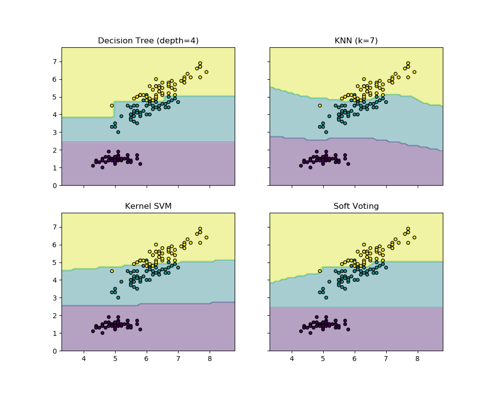
The following example illustrates how the decision regions may change when a soft VotingClassifier is used based on an linear Support Vector Machine, a Decision Tree, and a K-nearest neighbor classifier:下面的例子说明了在使用基于线性支持向量机、决策树和k近邻分类器的软投票分类器时,决策区域可能发生的变化:
from sklearn import datasets
from sklearn.tree import DecisionTreeClassifier
from sklearn.neighbors import KNeighborsClassifier
from sklearn.svm import SVC
from itertools import product
from sklearn.ensemble import VotingClassifier

# Loading some example data
iris = datasets.load_iris()
X = iris.data[:, [0, 2]]
y = iris.target

# Training classifiers
clf1 = DecisionTreeClassifier(max_depth=4)
clf2 = KNeighborsClassifier(n_neighbors=7)
clf3 = SVC(gamma='scale', kernel='rbf', probability=True)
eclf = VotingClassifier(estimators=[('dt', clf1), ('knn', clf2), ('svc', clf3)],
                        voting='soft', weights=[2, 1, 2])

clf1 = clf1.fit(X, y)
clf2 = clf2.fit(X, y)
clf3 = clf3.fit(X, y)
eclf = eclf.fit(X, y)
5.3 Using the VotingClassifier with GridSearch对投票分类器进行网格搜索
The VotingClassifier can also be used together with GridSearch in order to tune the hyperparameters of the individual estimators:VotingClassifier还可以与GridSearch一起使用,以优化单个估计器的超参数:
from sklearn.model_selection import GridSearchCV
clf1 = LogisticRegression(solver='lbfgs', multi_class='multinomial',
                          random_state=1)
clf2 = RandomForestClassifier(random_state=1)
clf3 = GaussianNB()
eclf = VotingClassifier(estimators=[('lr', clf1), ('rf', clf2), ('gnb', clf3)], voting='soft')

params = {'lr__C': [1.0, 100.0], 'rf__n_estimators': [20, 200]}

grid = GridSearchCV(estimator=eclf, param_grid=params, cv=5)
grid = grid.fit(iris.data, iris.target)
5.3.1 Usage使用
In order to predict the class labels based on the predicted class-probabilities (scikit-learn estimators in the VotingClassifier must support predict_proba method):为了基于预测的类概率预测类标签(投票分类器中的scikit-learn估计器必须支持predict_proba方法)
eclf = VotingClassifier(estimators=[('lr', clf1), ('rf', clf2), ('gnb', clf3)], voting='soft')
Optionally, weights can be provided for the individual classifiers:可选地,可以为单个分类器提供权重:
eclf = VotingClassifier(estimators=[('lr', clf1), ('rf', clf2), ('gnb', clf3)],
                        voting='soft', weights=[2, 5, 1])
参考: