Adaboost1
sklearn文档介绍AdaBoostClassifier采用的算法是SAMME和SAMME.R,在多分类时候此两种算法相对Freund等AdaBoost发明人的原算法有优势,下文全文翻译SAMME和SAMME.R发明人论文,当然,遇有不懂的我将找资料再去了解。
1 Introduction介绍
Boosting has been a very successful technique for solving the two-class classification problem. It was first introduced by Freund & Schapire (1997), with their AdaBoost algorithm. In going from two-class to multi-class classification, most boosting algorithms have been restricted to reducing the multi-class classification problem to multiple two-class problems, e.g. Freund & Schapire (1997), Schapire (1997), Schapire & Singer (1999), Allwein, Schapire & Singer (2000), Friedman, Hastie & Tibshirani (2000), Friedman (2001).增强法是解决两分类分类问题的一种非常成功的方法。它最初是由Freund & Schapire(1997)和他们的AdaBoost算法引入的。在从两分类分类到多分类分类的过程中,大多数的推进算法都局限于将多分类分类问题简化为多个两分类问题,如Freund & Schapire (1997), Schapire (1997), Schapire & Singer (1999), Allwein, Schapire & Singer (2000), Friedman, Hastie & Tibshirani (2000), Friedman(2001)。
In this paper, we develop a new algorithm that directly extends the AdaBoost algorithm to the multi-class case without reducing it to multiple two-class problems. Similar to AdaBoost in the two-class case, this new algorithm combines weak classifiers and only requires the performance of each weak classifier be better than random guessing (rather than 1/2).在本文中,我们开发了一种新的算法,它直接将AdaBoost算法扩展到多分类情况下,而不将其缩减为多个两分类问题。与两分类情况下的AdaBoost类似,该算法结合了弱分类器,只要求每个弱分类器的性能优于随机猜测(比1/2好)。
We believe this new algorithm covers a significant gap in the literature, as it is statistically motivated by a novel multi-class exponential loss function. In addition, similar to the original AdaBoost algorithm for the two-class classification, it fits a forward stagewise additive model.我们相信这个新算法在文献中有很大的空白,因为它是由一个新颖的多分类指数损失函数驱动的。此外,与原有的两分类分类AdaBoost算法相似,该算法适用于向前递归叠加模型。
As we will see, the new algorithm is extremely easy to implement, and is highly competitive with the best currently available multi-class classification methods, in terms of both practical performance and computational cost.正如我们将看到的,新算法非常容易实现,并且在实际性能和计算成本方面与当前可用的最佳多分类分类方法相比具有很强的竞争力。
1.1 AdaBoost
Before delving into the new algorithm for multi-class boosting, we briefly review the multi-class classification problem and the AdaBoost algorithm (Freund & Schapire 1997). Suppose we are given a set of training data $(\vec{x}_1,c_1),\ldots,(\vec{x}_n,c_n)$, where the input (predictor variable) $\vec{x}_i \in \mathbb{R}^p$, and the output (response variable) $c_i$ is qualitative and assumes values in a finite set, e.g. $\{1,2,\ldots,K\}$. $K$ is the number of classes. The goal is to find a classification rule $C(\vec{x})$ from the training data, so that when given a new input $\vec{x}$, we can assign it a class label $c$ from $\{1,2,\ldots,K\}$.在深入研究多分类增强的新算法之前,我们简要回顾了多分类分类问题和AdaBoost算法(Freund & Schapire 1997)。假设有训练数据$(\vec{x}_1,c_1),\ldots,(\vec{x}_n,c_n)$,其中输入(用于预测的变量)$\vec{x}_i \in \mathbb{R}^p$,和输出(回馈变量)$c_i$是定性的,并假设值在一个有限的集合,如$\{1,2,\ldots,K\}$。$K$是分类数。我们的目标是从训练数据中找到一个分类规则$C(\vec{x})$,这样当有一个新的输入$\vec{x}$时,我们就可以从$\{1,2,\ldots,K\}$中给它分配一个类标签$c$。
The question, then, is what is the best possible classification rule. To answer this question, we need to define what we mean by best. A common definition of best is to achieve the lowest misclassification error rate. Usually it is assumed that the training data are independently and identically distributed samples from an unknown probability distribution $Prob(\mathbf{X},C)$. Then the misclassification error rate for $C(\vec{x})$ is:那么,问题是什么是最好的分类规则。为了回答这个问题,我们需要定义什么是最好。常将达到最低误分类错误率定义为“好”。通常假设训练数据是来自未知概率分布$Prob(\mathbf{X},C)$的独立同分布样本。则$C(\vec{x})$的误分类错误率为:
$$\begin{align}
E_{\mathbf{X},C} \mathbb{I}_{C(\mathbf{X}) \ne C} &=E_{\mathbf{X}}Prob(C(\mathbf{X}) \ne C|\mathbf{X}) \\
&=1 −E_{\mathbf{X}} Prob(C(\mathbf{X})=C|\mathbf{X}) \\
&=1 − \sum_{k=1}^{K} E_{\mathbf{X}} [\mathbb{I}_{C(\mathbf{X})=k} Prob(C = k|\mathbf{X})]
\end{align} \tag{1}$$
即误分类率=1-正确分类率
It is clear that明显有
$$C^{∗}(\vec{x}) = \arg \max_{k} Prob(C = k|\mathbf{X} = \vec{x}) \tag{2}$$
will minimize this quantity with the misclassification error rate equal to $1−E_{\mathbf{X}} max_{k} Prob(C = k|\mathbf{X})$. This classifier is known as the Bayes classifier, and the error rate it achieves is the Bayes error rate.将最小化这个量使误分类错误率等于$1−E_{\mathbf{X}} max_{k} Prob(C = k|\mathbf{X})$。这个分类器被称为贝叶斯分类器,它所达到的错误率就是贝叶斯错误率。
贝叶斯分类器,依据$Prob(C = k|\mathbf{X} = \vec{x})$的最大概率分类数据点$\vec{x}$。同时,这等价于最小化误分类概率。
The AdaBoost algorithm is an iterative procedure that combines many weak classifiers to approximate the Bayes classifier $C^{∗}(\vec{x})$. Starting with the unweighted training sample, the AdaBoost builds a classifier, for example a classification tree (Breiman, Friedman, Olshen & Stone 1984), that produces class labels. If a training data point is misclassified, the weight of that training data point is increased (boosted). A second classifier is built using the new weights, which are no longer equal. Again, misclassified training data have their weights boosted and the procedure is repeated. Typically, one may build 500 or 1000 classifiers this way. A score is assigned to each classifier, and the final classifier is defined as the linear combination of the classifiers from each stage. Specifically, let $T(\vec{x})$ denote a weak multi-class classifier that assigns a class label to $\vec{x}$, then the AdaBoost algorithm proceeds as follows: AdaBoost算法是一个迭代过程,结合许多弱分类器来近似贝叶斯分类器$C^{∗}(\vec{x})$。从未加权的训练样本开始,AdaBoost构建一个分类器,例如生成类标签的分类树(Breiman, Friedman, Olshen & Stone 1984)。如果一个训练数据点分类错误,那么该训练数据点的权重就会增加。第二个分类器是使用不再相等的新权重构建的。再次,错误分类的训练数据会增加它们的权重,然后重复这个过程。通常,可以用这种方式构建500或1000个分类器。每个分类器都有一个分数,最终的分类器定义为每个阶段分类器的线性组合。具体地说,让$T(\vec{x})$表示一个弱的多分类分类器,该分类器将一个类标签赋给$\vec{x}$,然后AdaBoost算法进行如下操作:
Algorithm 1 AdaBoost (Freund & Schapire 1997)
- 1 Initialize the observation weights
$w_i =1/n, i =1 ,2,\ldots,n$. - 2 For
$m =1$to$M$:- (a) Fit a classifier
$T^{(m)}(\vec{x})$to the training data using weights$w_i$. - (b) Compute
$$err^{(m)} = \sum_{i=1}^{n}w_i \mathbb{I}(c_i \ne T^{(m)}(\vec{x}_i))/{\sum_{i=1}^{n}w_i} \tag{3}$$; if$err^{(m)} \ge 0.5$, stop and set$M = m − 1$. - (c) Compute
$$\alpha^{(m)} = \log \frac{1−err^{(m)}} {err^{(m)}} \tag{4}$$. - (d) Set
$$w_i \leftarrow w_i \cdot exp(\alpha^{(m)} \cdot \mathbb{I}(c_i \ne T^{(m)}(\vec{x}_i))), \\ i=1,2,\ldots,n \tag{5}$$. - (e) Re-normalize
$w_i$.
- (a) Fit a classifier
- 3 Output
$$C(\vec{x}) = \arg \max_{k} \sum_{m=1}^{M} \alpha^{(m)} \cdot \mathbb{I}(T^{(m)}(\vec{x})=k) \tag{6}$$由(4),分步分类器$f_k(\vec{x})$的权值$\alpha^{(m)}$取决于含权值$w_i$的样本的错误率$err^{(m)}$(注意错误率的计算不是根据这步的分类器本身,而是根据$1,\ldots,m$个分类器加权投票的集成分类器),错误率越大者,分步分类器的权值越大。从输出公式来看,分步分类器记为$\mathbb{I}(T^{(m)}(\vec{x})=k)$,说明其输出是分类本身而不是其概率,那么集成后的总分类器是通过加权投票的方式获得总的最终分类结果(权值为$\alpha^{(m)}$)。
When applied to two-class classification problems, AdaBoost has been proved to be extremely successful in producing accurate classifiers. In fact, Breiman (1996) called AdaBoost with trees the “best off-the-shelf classifier in the world.” However, it is not the case for multi-class problems, although AdaBoost was also proposed to be used in the multi-class case (Freund & Schapire 1997). Notice that in order for the misclassified training data to be boosted, it is required that the error of each weak classifier $err^{(m)}$ be less than 1/2 (with respect to the distribution on which it was trained), otherwise $\alpha^{(m)}$ will be negative and the weights of the training samples will be updated in the wrong direction in Algorithm 1 (2d). For two-class classification problems, this requirement is about the same as random guessing, but when K>2, accuracy 1/2 may be much harder to achieve than the random guessing accuracy rate 1/K. Hence, AdaBoost may fail if the weak classifier $T(\vec{x})$ is not chosen appropriately. To illustrate this point, we consider a simple three-class simulation example. Each input $\vec{x} \in \mathbb{R}^{10}$, and the ten input variables for all training examples are randomly drawn from a ten-dimensional standard normal distribution. The three classes are defined as:将AdaBoost算法应用于两分类分类问题中,取得了极好的分类效果。事实上,Breiman(1996)称树作为弱分类器的AdaBoost是世界上最好的现成分类器。然而,对于多分类问题却不是这样,尽管AdaBoost也被建议用于多分类问题(Freund & Schapire 1997)。需要注意的是,为了提高误分类的训练数据,需要每个弱分类器$err^{(m)}$的误差小于1/2(关于熟练数据的分布),否则$\alpha^{(m)}$将为负值并且算法1 (2d)中训练样本的权重将沿着错误的方向更新。对于两分类分类问题,这一要求与随机猜测差不多,但是当K>2时,准确率1/2可能比随机猜测准确率1/K更难达到。因此,如果弱分类器$T(\vec{x})$选择不当,AdaBoost可能会失败。为了说明这一点,我们考虑一个简单的三分类模拟示例。每个输入$\vec{x} \in \mathbb{R}^{10}$,以及所有训练例子的十个输入变量都是从一个十维标准正态分布中随机抽取的。
$$c = \begin{cases} 1, & \text{if $0 \le \sum x_{j}^{2} < \chi_{10,1/3}^{2}$,} \\ 2, & \text{if $\chi_{10,1/3}^{2} \le \sum x_{j}^{2} < \chi_{10,2/3}^{2},$} \\ 3, & \text{if $\chi_{10,2/3}^{2} \le \sum x_{j}^{2}$} \end{cases} \tag{7}$$
where $\chi_{10,k/3}^{2}$ is the (k/3)100% quantile of the $\chi_{10}^{2}$ distribution, so as to put approximately equal numbers of observations in each class. In short, the decision boundaries separating successive classes are nested concentric ten-dimensional spheres. The training sample size is 3000 with approximately 1000 training observations in each class. An independently drawn test set of 10000 observations is used to estimate the error rate.其中$\chi_{10,k/3}^{2}$是$\chi_{10}^{2}$分布的(k/3)100%分位数,所以在每一分类上都有大约相等的观察值。简而言之,分隔连续类的决策边界是嵌套的同心十维球体。训练样本量为3000,每个分类约1000个。采用独立抽样的10000个观测值的测试集来估计错误率。
Figure 1 (upper row) shows how AdaBoost breaks using ten-terminal node trees as weak classifiers. The results are averaged over ten independently drawn training-test set combinations. As we can see (upper left panel), the test error of AdaBoost decreases for a few iterations, then levels off around 0.53. What has happened can be understood from the upper middle and upper right panels: the $err^{(m)}$ starts below 0.5; after a few iterations, it overshoots 0.5($\alpha^{(m)}$ below 0), then quickly hinges onto 0.5. Once $err^{(m)}$ is equal to 0.5, the weights of the training samples do not get updated ($\alpha^{(m)}=0$), hence the same weak classifier is fitted over and over again but is not added to the existing fit, and the test error rate stays the same.图1(上行)显示了使用10个终端节点的树作为弱分类器的AdaBoost如何崩溃。结果平均自10个独立抽样的训练-测试集组合。正如我们所看到的(左上角的面板),AdaBoost的测试误差在几次迭代后会降低,然后在0.53左右趋于平稳。所发生的情况可以从上中和上右面板了解:$err^{(m)}$从0.5以下开始;经过一系列的迭代,它超过了0.5($\alpha^{(m)}$低于0),然后迅速固定到0.5。一旦$err^{(m)}$等于0.5,不更新训练样本的权重($\alpha^{(m)}=0$),因此相同的弱分类器训练一遍又一遍,但不能添加到现有的训练,并且测试错误率保持不变。
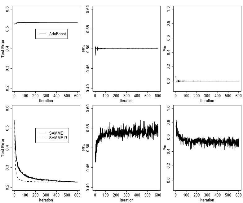 Figure 1: Comparison of AdaBoost and the new algorithm SAMME on a simple three-classsimulation example. The training sample size is 3000, and the testing sample size is 10000. Ten-terminal node trees are used as weak classifiers. The results are averaged over ten independently drawn training-test set combinations. The upper row is for AdaBoost and the lower row is for SAMME.AdaBoost算法与SAMME算法在一个简单的三分类实例上的比较。训练样本量为3000,测试样本量为10000。采用十个端节点的树作为弱分类器。结果来自对10个独立抽样的训练-测试集组合的平均。上行是AdaBoost结果,下行是SAMME结果。
1.2 Multi-class AdaBoost多分类AdaBoost
Before delving into technical details, we propose our new algorithm for multi-class boosting and compare it with AdaBoost. We refer to our algorithm as SAMME — Stagewise Additive Modeling using a Multi-class Exponential loss function — this choice of name will be clear in Section 2. Given the same setup as that of AdaBoost, SAMME proceeds as follows:在深入研究技术细节之前,我们提出了新的多分类增强算法,并与AdaBoost算法进行了比较。将算法命名为SAMME——使用多分类指数损失函数进行逐级加性建模,名字的选择将在第二节阐述。在与AdaBoost相同的步骤下,SAMME进行如下操作:
其权重更新公式根据Littlestone and Warmuth's weighted majority algorithm,见参考1第3页,推导过程见参考3第9页。严格说起来,因为权重更新公式不同,这不是完全意义上Freund & Schapire的算法。
Algorithm 2. SAMME (SAMME — Stagewise Additive Modeling using a Multi-class Exponential loss function)
- 1 Initialize the observation weights
$w_i =1/n, i =1 ,2,\ldots,n$. - 2 For
$m =1$to$M$:- (a) Fit a classifier
$T^{(m)}(\vec{x})$to the training data using weights$w_i$. - (b) Compute
$$err^{(m)} = \sum_{i=1}^{n}w_i \mathbb{I}(c_i \ne T^{(m)}(\vec{x}_i))/{\sum_{i=1}^{n}w_i}$$; if$err^{(m)} \ge 0.5$, stop and set$M = m − 1$. - (c) Compute
$$\alpha^{(m)} = \log \frac{1−err^{(m)}} {err^{(m)}} + \log (K-1) \tag{8}$$. - (d) Set
$$w_i \leftarrow w_i \cdot exp(\alpha^{(m)} \cdot \mathbb{I}(c_i \ne T^{(m)}(\vec{x}_i))), \\ i=1,2,\ldots,n$$. - (e) Re-normalize
$w_i$.
- (a) Fit a classifier
- 3 Output
$$C(\vec{x}) = \arg \max_{k} \sum_{m=1}^{M} \alpha^{(m)} \cdot \mathbb{I}(T^{(m)}(\vec{x})=k)$$由(8),分步分类器$f_k(\vec{x})$的权值$\alpha^{(m)}$取决于含权值$w_i$的样本的错误率$err^{(m)}$(注意错误率的计算不是根据这步的分类器本身,而是根据$1,\ldots,m$个分类器加权投票的集成分类器),错误率越大者,分步分类器的权值越大。从输出公式来看,分步分类器记为$\mathbb{I}(T^{(m)}(\vec{x})=k)$,说明其输出是分类本身而不是其概率,那么集成后的总分类器是通过加权投票的方式获得总的最终分类结果(权值为$\alpha^{(m)}$)。
Notice Algorithm 2 (SAMME) is very similar to AdaBoost with a major difference in (8). Now in order for $\alpha^{(m)}$ to be positive, we only need $(1−err^{(m)}) > 1/K$, or the accuracy of each weak classifier be better than random guessing rather than 1/2. As a consequence, the new algorithm puts more weight on the misclassified data points in (2d) than AdaBoost, and the new algorithm also combines weak classifiers a little differently from AdaBoost, i.e. differ by $\log (K −1) \sum_{m=1}^{M} \mathbb{I}(T^{(m)}(\vec{x})=k)$. It is worth noting that when $K = 2$, SAMME reduces to AdaBoost. As we will see in Section 2, the extra term $\log (K −1)$ in (8) is not artificial; it makes the new algorithm equivalent to fitting a forward stagewise additive model using a multi-class exponential loss function. The difference between AdaBoost and SAMME (when $K = 3$) is also illustrated in Figure 1. As we have seen (upper left panel), AdaBoost breaks after the $err^{(m)}$ goes above 1/2. However this is not the case for SAMME (lower row): although $err^{(m)}$ can be bigger than 1/2 (or equal to 1/2), the $\alpha^{(m)}$ is still positive; hence, the mis-classified training samples get more weights, and the test error keeps decreasing even after 600 iterations.注意算法2 (SAMME)与AdaBoost非常相似,但在(8)方面有很大的不同。现为使$\alpha^{(m)}$为正值,只需$(1−err^{(m)}) > 1/K$(在(8)中直接令$\alpha^{(m)}>0$即可得到。),或者每个弱分类器的准确率都优于随机猜测而不是1/2(当$K = 2$时,在(8)中直接令$\alpha^{(m)}>0$即可得到$(1−err^{(m)}) > 1/K = 1/2$。)。随即,新算法在(2d)比AdaBoost对误分类的数据点赋予更多权值,而且新算法组合弱分类器也与AdaBoost稍有不同,也就是差异为$\log (K −1) \sum_{m=1}^{M} \mathbb{I}(T^{(m)}(\vec{x})=k)$。值得注意的是,当$K = 2$时,SAMME会退化为AdaBoost。正如我们将在第2节中看到的,(8)中的额外项$\log (K −1)$不是人工的;它使得新算法等价于使用一个多分类指数损失函数拟合一个向前递归叠加模型。AdaBoost和SAMME(当$K = 3$)之间的区别也如图1所示。正如我们所看到的(上左面板),$err^{(m)}$大于1/2之后,AdaBoost崩溃。然而对SAMME(下行)情况并非如此:虽然$err^{(m)}$可以大于1/2(或等于1/2),$\alpha^{(m)}$仍然是正值;因此,分类错误的训练样本得到了更多的权重,即使经过600次迭代,测试误差也在不断减小。
The rest of the paper is organized as follows: In Section 2 and 3, we give theoretical justification for our new algorithm SAMME. In Section 4, we present numerical results on both simulation and real-world data. Summary and discussion regarding the implications of the new algorithm are in Section 5.本文的其余部分组织如下:在第2节和第3节中,我们对我们的新算法SAMME进行了理论论证。在第4节中,我们给出了模拟数据和真实数据的数值结果。关于新算法的含义的总结和讨论在第5节中。
2 Theoretical Justification理论依据
In this section, we are going to show that the extra term log(K − 1) in (8) is not artificial; it makes Algorithm 2 equivalent to fitting a forward stagewise additive model using a multi-class exponential loss function. Friedman et al. (2000) developed a statistical perspective on the original two-class AdaBoost algorithm, which ultimately leads to viewing the two-class AdaBoost algorithm as forward stagewise additive modeling using the exponential loss function在这一节中,我们将证明(8)中的额外项log(K − 1)不是人工的;这使得算法2等价于使用一个多分类指数损失函数来拟合一个向前递归叠加模型。Friedman et al.(2000)对原有的两分类AdaBoost算法进行了统计分析,最终将两分类AdaBoost算法视为使用指数损失函数的向前递归叠加建模
$$L(y,f)=e^{−yf(\vec{x})} \tag{9}$$,
where $y =(\mathbb{I}(c = 1)− \mathbb{I}(c = 2)) \in \{− 1,1\}$ in a two-class classification setting. It is not difficult to show that the population minimizer of this exponential loss function is one half of the logit transform其中对两分类设定有$y =(\mathbb{I}(c = 1)− \mathbb{I}(c = 2)) \in \{− 1,1\}$。不难看出,这个指数损失函数的总体最小值是logit变换的一半
$$\begin{align}
f^*(\vec{x}) & = \arg\min_{f(\vec{x})} L(y,f) \\
& = \frac{1} {2} \log \frac{Prob(c =1 |\vec{x})} {Prob(c =2 |\vec{x})}
\end{align} \tag{10}$$
$$\begin{align}
f^*(\vec{x}) & = \arg\min_{f(\vec{x})} L(y,f) \\
& = \frac{1} {2} \log \frac{Prob(c =1 |\vec{x})} {Prob(c =2 |\vec{x})} \\
& = \frac{1} {2} \left(\log Prob(c =1 |\vec{x}) - \log Prob(c =2 |\vec{x})\right)
\end{align}$$
?????????
. The Bayes optimal classification rule then agrees with the sign of $f^∗(\vec{x})$, i.e.则贝叶斯最优分类规则与$f^∗(\vec{x})$符号一致,即
$$\arg \max_{y} Prob(Y = y|\vec{X} = \vec{x}) = sign(f^∗(\vec{x})) \tag{11}$$
. We note that besides Friedman et al. (2000), Breiman (1999) and Schapire & Singer (1999) also made connections between the original two-class AdaBoost algorithm and the exponential loss function. We acknowledge that these views have been influential in our thinking for this paper.我们注意到,除了Friedman et al. (2000), Breiman(1999)和Schapire & Singer(1999)也将原来的两分类AdaBoost算法与指数损失函数联系起来。我们承认这些观点对我们撰写本文的思路产生了影响。
2.1 A new multi-class exponential loss function新的多分类指数损失函数
In the multi-class classification setting, we can recode the output $c$ with a $k$-dimensional vector $\vec{y}$, with all entries equal to $− \frac{1} {K−1}$ except a 1 in position $k$ if $c = k$, i.e. $\vec{y} =( y_1,\ldots,y_K)^T$, and:在多分类分类设置中,我们可以用$k$维向量$\vec{y}$来重新编码输出$c$。如果$c = k$,那么位置$k$为1,除此以外所有位置都等于$− \frac{1} {K−1}$,即$\vec{y} =( y_1,\ldots,y_K)^T$,并且
$$y_k = \begin{cases} 1, & \text{if $c=k$} \\ − \frac{1} {K−1}, & \text{if $c \ne k$} \end{cases} \tag{12}$$ ,
Lee, Lin & Wahba (2004) used the same coding for a version of the multi-class support vector machine. A generalization of the exponential loss function to the multi-class case then follows naturally: Lee, Lin和Wahba(2004)对多分类支持向量机的一个版本使用了相同的编码。指数损失函数在多分类情况下的自然推广为
$$L(\vec{y},\vec{f}) = \exp \left(− \frac{1} {K} (y_1f_1 +\dots+ y_Kf_K)\right)= \exp \left(− \frac{1} {K} \vec{y} \vec{f}\right) \tag{13}$$
where $f_k$ corresponds to class $k$, and its meaning will be clear shortly. Notice that we need some constraint on $\vec{f}$ in order for it to be estimable, otherwise adding any constant to all $f_k$’s does not change the loss. We choose to use the symmetric constraint: $f_1 +\dots+ f_K = 0$, so when $K = 2$, this multi-class exponential loss function reduces to the two-class exponential loss.其中$f_k$对应分类$k$,其含义很快就会清楚。注意,我们需要对$\vec{f}$进行一些约束,以使其可估计,否则在所有$f_k$中添加任何常数都不会改变损失。我们选择使用对称约束:$f_1 +\dots+ f_K = 0$,因此当$K = 2$时,这个多分类指数损失函数会退化为两分类指数损失。
Similar to the two-class case, it is of interest to investigate what this multi-class exponential loss function estimates. This can be answered by seeking its population minimizer. Specifically, we are interested in与两分类情况类似,研究这个多分类指数损失函数的估计值也很有趣。这可以通过寻求其总体最小值来解决。具体来说,我们感兴趣的是
$$\begin{align}
\arg \min_{\vec{f}(\vec{x})} & \quad E_{\mathbf{Y}|\vec{x}} \exp \left(− \frac{1} {K} (y_1f_1 +\dots+ y_Kf_K)\right) \\
\text{subject to} & \quad f_1 +\dots+ f_K =0 .
\end{align} \tag{14}$$
The Lagrange of this constrained optimization problem can be written as:这个约束优化问题的拉格朗日函数可以写成:
$$\exp \left(−\frac {f_1(\vec{x})} {K −1}\right)Prob(c =1 |\vec{x})+\dots+\exp \left(−\frac {f_K(\vec{x})} {K−1}\right)Prob(c =K |\vec{x}) \\−\lambda(f_1(\vec{x})+\dots+ f_K(\vec{x})), \tag{15}$$
也就是$$E_{\mathbf{Y}|\vec{x}} \exp \left(− \frac{1} {K} (y_1f_1 +\dots+ y_Kf_K)\right)−\lambda(f_1(\vec{x})+\dots+ f_K(\vec{x}))$$,详情请百度拉格朗日乘子法。
where $\lambda$ is the Lagrange multiplier. Taking derivatives with respect to $f_k$ and $\lambda$, we reach其中,$\lambda$是拉格朗日乘子。对$f_k$和$\lambda$求导,我们得到
$$\begin{align}
\frac{1}{K −1}\exp \left(−\frac {f_1(\vec{x})} {K −1}\right)Prob(c =1 |\vec{x})−\lambda &=0,\\
\vdots \\
\frac{1}{K −1}\exp \left(−\frac {f_K(\vec{x})} {K −1}\right)Prob(c =K |\vec{x})−\lambda &=0,\\
f_1(\vec{x})+\dots+f_K(\vec{x}) &=0.
\end{align} \tag{16}$$
Solving this set of equations, we obtain the population minimizer解这组方程,我们得到总体最小值
$$f_k^∗(\vec{x})=(K −1)\left(\log Prob(c = k|\vec{x})− \frac{1} {K} \sum_{k'=1}^{K} \log Prob(c = k'|\vec{x})\right),\\ \quad k=1,...,K. \tag{17}$$
解联立等式组(46)得$$\frac{1} {K} \sum_{k'=1}^{K} \log Prob(c = k'|\vec{x})=\log [(K-1)\lambda]$$然后可以得到上式。
Thus,因此
$$\arg \max_k f_k^∗(\vec{x}) = \arg \max_k Prob(c = k|\vec{x}) \tag{18}$$
(17)可改写为$$f_k^∗(\vec{x})=(K −1)\left(\frac{K-1} {K}\log Prob(c = k|\vec{x})− \frac{1} {K} (\log Prob(c = 1|\vec{x})+\cdots\\
+\log Prob(c = k-1|\vec{x})+\log Prob(c = k+1|\vec{x})+\cdots+\log Prob(c = K|\vec{x}))\right)$$显然,$Prob(c = k|\vec{x})$与$f_k^∗(\vec{x})$最大化将取得相同的$k$。
which is the Bayes optimal classification rule in terms of minimizing the misclassification error. This justifies the use of this multi-class exponential loss function. Equation (17) also provides a way to recover the class probability $Prob(c = k|\vec{x})$ once $f_k^∗(\vec{x})$’s are estimated, i.e.这是最小化误分类误差的贝叶斯最优分类规则。这证明了使用多分类指数损失函数的合理性。等式(17)也提供了根据$f_k^∗(\vec{x})$概率得到$Prob(c = k|\vec{x})$的一个方法,即
$$Prob(c = k|\vec{x})= \frac{e ^ {\frac{1} {K−1} f_k^∗(\vec{x})}} {e ^ {\frac{1} {K−1} f_1^∗(\vec{x})}+\dots+e ^ {\frac{1} {K−1} f_K^∗(\vec{x})}},k=1,...,K. \tag{19}$$
显然联立(17)无法得到(19)。但是,当$\vec{x}$被正确分类到某个$k$,那么$\log Prob(c = k|\vec{x})$远大于其余log概率,也远大于$\frac{1} {K} \sum_{k'=1}^{K} \log Prob(c = k'|\vec{x})$,那么$f_k^∗(\vec{x}) \approx (K −1)\left(\log Prob(c = k|\vec{x})\right)$。即$Prob(c = k|\vec{x})= e ^ {\frac{1} {K−1} f_k^∗(\vec{x})}$,显然$\sum_{k=1}^{K}Prob(c = k|\vec{x})=1$,归一化即得到(19)。
2.2 Forward stagewise additive modeling前项逐步叠加模型
We now show that Algorithm 2 is equivalent to forward stagewise additive modeling using the loss function (32). We start with the forward stagewise additive modeling using a general loss function $L(·,·)$, then apply it to the multi-class exponential loss function (32). Given the training data, we wish to find $\vec{f}(\vec{x})=( f_1(\vec{x}),\ldots,f_K(\vec{x}))^T$ such that我们现在证明算法2等价于使用损失函数(32)进行向前递归叠加建模。我们从使用一般损失函数$L(·,·)$的正向前递归叠加建模开始,然后将其应用于多分类指数损失函数(32)。给定训练数据,我们希望找到$\vec{f}(\vec{x})=( f_1(\vec{x}),\ldots,f_K(\vec{x}))^T$以使
$$\begin{align}
\min_{f(\vec{x})} & \quad \sum_{i=1}^{n} L(\vec{y}_i,\vec{f}(\vec{x}_i)) \tag{20}\\
\text{subject to} & \quad f_1(\vec{x})+\dots+ f_K(\vec{x})=0 . \tag{21}
\end{align}$$
We consider $\vec{f}(\vec{x})$ that has the following form:我们考虑$\vec{f}(\vec{x})$具有以下形式:
$$\vec{f}(\vec{x})= \sum_{m=1}^{M} \beta^{(m)}\vec{g}^{(m)}(\vec{x}), \tag{22}$$
where $\beta^{(m)} \in \mathbb{R}$ are coefficients, and $\vec{g}^{(m)}(\vec{x})$ are basis functions. We require $\vec{g}(\vec{x})$ to satisfy the symmetric constraint: $g_1(\vec{x})+\dots+ g_K(\vec{x})=0$其中$\beta^{(m)} \in \mathbb{R}$是系数,并且$\vec{g}^{(m)}(\vec{x})$是基函数。要求$\vec{g}(\vec{x})$满足对称约束
$$g_1(\vec{x})+\dots+g_K(\vec{x})=0 \tag{23}$$
For example, the $\vec{g}(\vec{x})$ that we consider in this paper takes value in one of the $K$ possible $K$-dimensional vectors in (31); specifically, at a given $\vec{x}$, $\vec{g}(\vec{x})$ mapps $\vec{x}$ onto $\mathbf{Y}$:例如,本文考虑的$\vec{g}(\vec{x})$取值等式(31)中$K$维向量中的$K$个可能值中的一个;进一步,对一给定$\vec{x}$,$\vec{g}(\vec{x})$映射$\vec{x}$到$\mathbf{Y}$:
$$\vec{g} : \vec{x} \in \mathbb{R}^p \rightarrow \mathbf{Y}$$
注意,每个$\vec{x}$其实只映射到$\mathbf{Y}$中其中一个行向量。
, where $\mathbf{Y}$ is the set containing $K$ $K$-dimensional vectors:其中$\mathbf{Y}$是一包含$K$个$K$维向量的集合:
$$\mathbf{Y} = \begin{Bmatrix}
\left(1,-\frac{1}{K-1},\ldots,-\frac{1}{K-1}\right)^T \\
\left(-\frac{1}{K-1},1,\ldots,-\frac{1}{K-1}\right)^T \\
\vdots \\
\left(-\frac{1}{K-1},-\frac{1}{K-1},\ldots,1\right)^T
\end{Bmatrix} \tag{24}$$
Forward stagewise modeling approximates the solution to (20) – (21) by sequentially adding new basis functions to the expansion without adjusting the parameters and coefficients of those that have already been added. Specifically, the algorithm starts with $\vec{f}^{(0)}(\vec{x}) = 0$, sequentially selecting new basis functions from a dictionary and adding them to the current fit:向前逐步模型通过在展开中依次添加新的基函数,而不调整已经添加的基函数的参数和系数,近似于(20)-(21)的解(为什么是近似,因为基函数是弱分类器,其并不要求无限发育的树从而得到全局最优。)。具体来说,算法从$\vec{f}^{(0)}(\vec{x}) = \vec{0}$开始,从字典中顺序选择新基函数并将之加进当前训练:
Algorithm 3 Forward stagewise additive modeling
- 1 Initialize
$\vec{f}^{(0)}(\vec{x}) = \vec{0}$. - 2 For
$m=1$to$M$:- (a) Compute
$$(\beta^{(m)},\vec{g}^{(m)}(\vec{x})) = \arg \min_{\beta,\vec{g}} \sum_{i=1}^{n} L(\vec{y}_i,\vec{f}^{(m-1)}(\vec{x}_i)+\beta \vec{g}(\vec{x}_i)) \tag{25}$$. - (b) Set
$$\vec{f}^{(m)}(\vec{x})=\vec{f}^{(m-1)}(\vec{x})+\beta^{(m)}\vec{g}^{(m)}(\vec{x}) \tag{26}$$.
- (a) Compute
The crucial step in the above algorithm is (2a). Now, using the multi-class exponential loss function (32), one wants to find $\vec{g}^{(m)}(\vec{x})$ (and $\beta^{(m)}$) to solve:上述算法的关键步骤是(2a)。现在,使用多分类指数损失函数(32),解如下方程来找到$\vec{g}^{(m)}(\vec{x})$(还有$\beta^{(m)}$):
$$\begin{align}
(\beta^{(m)},\vec{g}^{(m)}(\vec{x})) & = \arg \min_{\beta,\vec{g}} \sum_{i=1}^{n} \exp \left(− \frac{1} {K} \vec{y}_i^T (\vec{f}^{(m-1)}(\vec{x}_i)+\beta \vec{g}(\vec{x}_i))\right) \tag{27} \\
& = \arg \min_{\beta,\vec{g}} \sum_{i=1}^{n} w_i \exp \left(− \frac{1} {K} \beta \vec{y}_i^T \vec{g}(\vec{x}_i)\right), \tag{28}
\end{align}$$
where $w_i = \exp \left(− \frac{1} {K} \vec{y}_i^T \vec{f}^{(m-1)}(\vec{x}_i)\right)$ are the unnormalized observation weights.其中$w_i = \exp \left(− \frac{1} {K} \vec{y}_i^T \vec{f}^{(m-1)}(\vec{x}_i)\right)$为未归一化观测权值。
Notice that every $\vec{g}(\vec{x})$ as in (24) has a one-to-one correspondence with a multi-class classifier $T(\vec{x})$ in the following way:注意,(24)中的每一个$\vec{g}(\vec{x})$都以以下方式与多分类分类器$T(\vec{x})$一一对应:
$$T(\vec{x})=k,\ if \ g_k(\vec{x})=1 \tag{29}$$
and vice versa:反之亦然:
$$g_k(\vec{x}) = \begin{cases} 1, & \text{if $T(\vec{x})=k$,} \\ -\frac{1}{K−1}, & \text{if $T(\vec{x}) \ne k$.} \end{cases} \tag{30}$$
Hence, solving for $\vec{g}^{(m)}(\vec{x})$ in (28) is equivalent to finding the multi-class classifier $T^{(m)}(\vec{x})$ that can generate $\vec{g}^{(m)}(\vec{x})$.因此,求解(28)中的$\vec{g}^{(m)}(\vec{x})$等价于找到能够生成$\vec{g}^{(m)}(\vec{x})$的多分类分类器$T^{(m)}(\vec{x})$。
Lemma 1 The solution to (28) is引理1 (28)的解是
$$\begin{align}
T^{(m)}(\vec{x}) &= \arg \min \sum_{i=1}^{n}
w_i \mathbb{I}(c_i \ne T(\vec{x}_i)), \tag{31} \\
\beta^{(m)} &=
\frac{(K −1)^2} {K} \left(\log \frac{1−err^{(m)}} {err^{(m)}}
+\log(K −1)\right), \tag{32}
\end{align}$$
where $err^{(m)}$ is defined as其中$err^{(m)}$定义如下:
$$err^{(m)} = \sum_{i=1}^{n} \mathbb{I}(c_i \ne T(\vec{x}_i)) / \sum_{i=1}^{n} w_i \tag{33}$$
Proof First, for any fixed value of $\beta > 0$, using the definition (29), one can express the criterion in (28) as:先证明,对于$\beta > 0$的任何固定值,使用定义(29),可以将(28)中的标准表示为:
$$\begin{align}
& \sum_{c_i = T(\vec{x}_i)} w_i e^{-\frac{\beta}{K-1}} + \sum_{c_i \ne T(\vec{x}_i)} w_i e^{\frac{\beta}{(K-1)^2}} \\
= & e^{-\frac{\beta}{K-1}} \sum_{i=1}^{n} w_i + (e^{\frac{\beta}{(K-1)^2}} - e^{-\frac{\beta}{K-1}}) \sum_{i=1}^{n} w_i \mathbb{I}(c_i \ne T(\vec{x}_i))
\end{align} \tag{34}$$
根据(12)和(30)可以从(28)得到(34)第一行,然后
$$\begin{align}
& \sum_{c_i = T(\vec{x}_i)} w_i e^{-\frac{\beta}{K-1}} + \sum_{c_i \ne T(\vec{x}_i)} w_i e^{\frac{\beta}{(K-1)^2}} \\
= & e^{-\frac{\beta}{K-1}} \sum_{c_i = T(\vec{x}_i)} w_i + e^{\frac{\beta}{(K-1)^2}} \sum_{c_i \ne T(\vec{x}_i)} w_i \\
= & e^{-\frac{\beta}{K-1}} \sum_{i=1}^{n} w_i - e^{-\frac{\beta}{K-1}} \sum_{c_i \ne T(\vec{x}_i)} w_i + e^{\frac{\beta}{(K-1)^2}} \sum_{c_i \ne T(\vec{x}_i)} w_i \\
= & e^{-\frac{\beta}{K-1}} \sum_{i=1}^{n} w_i + (e^{\frac{\beta}{(K-1)^2}} - e^{-\frac{\beta}{K-1}}) \sum_{c_i \ne T(\vec{x}_i)} w_i \\
= & e^{-\frac{\beta}{K-1}} \sum_{i=1}^{n} w_i + (e^{\frac{\beta}{(K-1)^2}} - e^{-\frac{\beta}{K-1}}) \sum_{i=1}^{n} w_i \mathbb{I}(c_i \ne T(\vec{x}_i))
\end{align}$$
Since only the last sum depends on the classifier $T(\vec{x})$, we get that (31) holds. Now plugging (31) into (28) and solving for $\beta$, we obtain (32) (note that (34) is a convex function of $\beta$).既然只有后项求和依赖分类器$T(\vec{x})$,我们知道(31)成立。现将(31)插入(28)中来求解$\beta$,我们得到(32)(注意(34)是$\beta$的凸函数)。
对(34)关于$\beta$求偏导并令偏导数为0,得:$$[\frac{1}{(K-1)^2} e^{\frac{\beta}{(K-1)^2}} + \frac{1}{K-1} e^{-\frac{\beta}{K-1}}] \sum_{i=1}^{n} w_i \mathbb{I}(c_i \ne T(\vec{x}_i)) - \frac{1}{K-1} e^{-\frac{\beta}{K-1}} \sum_{i=1}^{n} w_i = 0$$乘以${(K-1)}^2$得$$[e^{\frac{\beta}{(K-1)^2}} + (K-1) e^{-\frac{\beta}{K-1}}] \sum_{i=1}^{n} w_i \mathbb{I}(c_i \ne T(\vec{x}_i)) - (K-1) e^{-\frac{\beta}{K-1}} \sum_{i=1}^{n} w_i = 0$$乘以$e^{\frac{\beta}{K-1}}$得$$[e^{\frac{\beta}{(K-1)^2} + \frac{\beta}{K-1}} + (K-1)] \sum_{i=1}^{n} w_i \mathbb{I}(c_i \ne T(\vec{x}_i)) - (K-1) \sum_{i=1}^{n} w_i = 0$$移项得$$\begin{align} & e^{\frac{K\beta}{(K-1)^2}}\\ = &\frac{(K-1)(\sum_{i=1}^{n} w_i - \sum_{i=1}^{n} w_i \mathbb{I}(c_i \ne T(\vec{x}_i)))}{\sum_{i=1}^{n} w_i \mathbb{I}(c_i \ne T(\vec{x}_i))}\\=&\frac{(K-1)(1-err^{(m)})}{err^{(m)}}\end{align}$$再两边取对数即可得到(32)。
The model is then updated然后模型更新
$$\vec{f}^{(m)}(\vec{x})=\vec{f}^{(m-1)}(\vec{x})+\beta^{(m)}\vec{g}^{(m)}(\vec{x}) \tag{35}$$
, and the weights for the next iteration will be并且下一轮迭代的权值将会是
$$w_i \leftarrow w_i \cdot \exp \left(-\frac{1}{K}\beta^{(m)} \vec{y}_i^T \vec{g}^{(m)}(\vec{x})\right) \tag{36}$$
(36)是求$m+1$步基函数所需的样本权值,从中我们得出这样的结论:权值更新系数就是标签和上步基函数对应的损失,权值就是标签和上步为止的集成函数对应的损失。
. This is equal to这等于
$$w_i \cdot e^ {-\frac{(K-1)^2}{K^2}\alpha^{(m)} \vec{y}_i^T \vec{g}^{(m)}(\vec{x})} = \begin{cases} w_i \cdot e^ {-\frac{K-1}{K}\alpha^{(m)}}, & \text{if $c_i = T(\vec{x}_i)$} \\ w_i \cdot e^ {\frac{1}{K}\alpha^{(m)}}, & \text{if $c_i \ne T(\vec{x}_i)$} \end{cases} \tag{37}$$
根据(12)和(30)即可得到上式。
where $\alpha^{(m)}$ is defined as in (8) with the extra term $\log (K−1)$, and the new weight (37) is equivalent to the weight updating scheme in Algorithm 2 (2d) after normalization.其中$\alpha^{(m)}$在(8)中已定义并包含额外项$\log (K−1)$,新的权值(37)相当于算法2 (2d)更新的权值经过归一化。
考虑(37)中两种情况同时乘以$N^{(m)}$,并按SAMME算法,正确分类的不更新权值。即$w_i \cdot e^ {-\frac{K-1}{K}\alpha^{(m)}} \cdot N^{(m)}=w_i$,则$N^{(m)}=e^ {\frac{K-1}{K}\alpha^{(m)}}$,那么$w_i \cdot e^ {\frac{1}{K}\alpha^{(m)}} \cdot N^{(m)}=w_i \cdot e^ {\alpha^{(m)}}$,即(8)成立。
It is also a simple task to check that $\arg \max_{k} \vec{f}^{(m)}(\vec{x}) = \arg \max_{k} (f_{1}^{(m)}(\vec{x}),...,f_{K}^{(m)}(\vec{x}))^T$ is equivalent to the output $C(\vec{x}) = \arg \max_{k} \sum_{m=1}^{M} \alpha^{(m)} \cdot \mathbb{I}(T^{(m)}(\vec{x})=k)$$ in Algorithm 2. Hence, Algorithm 2 can be considered as forward stagewise additive modeling using the multi-class exponential loss function.检查$\arg \max_{k} \vec{f}^{(m)}(\vec{x}) = \arg \max_{k} (f_{1}^{(m)}(\vec{x}),...,f_{K}^{(m)}(\vec{x}))^T$等价于算法2的输出$C(\vec{x}) = \arg \max_{k} \sum_{m=1}^{M} \alpha^{(m)} \cdot \mathbb{I}(T^{(m)}(\vec{x})=k)$也是容易的(贝叶斯规则,正确分类取概率最大者。)。因此,可以将算法2考虑为使用多分类指数损失函数的向前递归叠加建模。
2.3 Computational cost计算复杂度
Suppose one uses a classification tree as the weak learner, which is the most popular choice, and the depth of each tree is fixed as $d$, then the computational cost for building each tree is $O(dpnlog(n))$, where $p$ is the dimension of the input $\vec{x}$. The computational cost for our SAMME algorithm is then $O(dpnlog(n)M)$ since there are $M$ iterations. As a comparison, the computational cost for either the one vs. rest scheme or the pairwise scheme (Friedman 2004) is $O(dpnlog(n)MK)$, which is $K$ times larger than the computational cost of SAMME.假设使用分类树作为弱学习器,这是最流行的选择,每棵树的深度固定为$d$,那么构建每棵树的计算成本为$O(dpnlog(n))$,其中$p$是输入$\vec{x}$的维度。我们的SAMME算法的计算成本是$O(dpnlog(n)M)$,因为有$M$迭代。作为比较,对于一对多方案或成对方案(Friedman 2004),计算成本都是$O(dpnlog(n)MK)$,即比SAMME的计算成本大$K$倍。
3 A Variant of the SAMME Algorithm SAMME算法的一个变体
The SAMME algorithm expects the weak learner to deliver a classifier $T(\vec{x}) \in \{ 1,\ldots,K\}$. An alternative is to use real-valued confidence-rated predictions such as weighted probability estimates, to update the additive model, rather than the classifications themselves.SAMME算法期望从弱学习器得到一个分类器$T(\vec{x}) \in \{ 1,\ldots,K\}$。另一种方法是使用实值信心评级预测(如加权概率估计)来更新叠加模型,而不是使用分类本身。
Section 2.2 is based on the empirical loss, this time we consider the population version of the loss, derive the update for the additive model using the weighted probability, and then apply it to data.第2.2节基于经验损失,本次我们考虑损失的总体版本,利用加权概率对叠加模型进行更新,并将其应用于数据。
Suppose we have a current estimate $\vec{f}^{(m−1)}(\vec{x})$ and seek an improved estimate $\vec{f}^{(m−1)}(\vec{x})+\vec{h}(\vec{x})$ by minimizing the loss at each $\vec{x}$:假设目前估计器为$\vec{f}^{(m−1)}(\vec{x})$,通过每个$\vec{x}$来最小化损失以得到一个改进的估计器:
$$\begin{align}
min_{\vec{h}(\vec{x})} & \quad E\left(exp\left(-\frac{1}{K} \vec{y}^T (\vec{f}^{(m−1)}(\vec{x})+\vec{h}(\vec{x}))\right)|\vec{x}\right) \\
\text{subject to} & \quad h_1(\vec{x})+\dots+h_K(\vec{x})=0
\end{align} \tag{38}$$
The above expectation can be re-written as上式期望可改写为
$$\begin{align}
& e^{-\frac{h_1(\vec{x})}{K-1}} E\left(e^{-\frac{1}{K} \vec{y}^T \vec{f}^{(m−1)}(\vec{x})} \mathbb{I}_{c=1}|\vec{x}\right)+\dots+e^{-\frac{h_K(\vec{x})}{K-1}} E\left(e^{-\frac{1}{K} \vec{y}^T \vec{f}^{(m−1)}(\vec{x})} \mathbb{I}_{c=K}|\vec{x}\right) \\
= & e^{-\frac{h_1(\vec{x})}{K-1}} Prob_w(c=1|\vec{x})+\dots+e^{-\frac{h_1(\vec{x})}{K-1}} Prob_w(c=K|\vec{x})
\end{align} \tag{39}$$
where $w(\vec{x},\vec{y}) = \exp (− \frac{1} {K} \vec{y}^T \vec{f}^{(m−1)}(\vec{x}))$, and其中$w(\vec{x},\vec{y}) = \exp (− \frac{1} {K} \vec{y}^T \vec{f}^{(m−1)}(\vec{x}))$,并且:
$$Prob_w(c = k|\vec{x})=E\left(e^{− \frac{1} {K} \vec{y}^T \vec{f}^{(m−1)}(\vec{x})} \mathbb{I}_{c=k}|\vec{x}\right) \tag{40}$$
Taking the symmetric constraint into consideration and optimizing the Lagrange will lead to the solution (details skipped)考虑对称约束并优化拉格朗日方程将得到解决方案(跳过细节)
$$h_k(\vec{x})=(K −1)\left(\log Prob_w(c = k|\vec{x})− \frac{1} {K} \sum_{k'=1}^{K} \log Pro_w(c = k'|\vec{x})\right) \tag{41}$$
联合(38)和(39)并运用拉格朗日乘子法得(类比(46)):
$$\begin{align}
\frac{1}{K −1}\exp \left(−\frac {h_1(\vec{x})} {K −1}\right)Prob_w (c =1 |\vec{x})−\lambda &=0,\\
\vdots \\
\frac{1}{K −1}\exp \left(−\frac {h_K(\vec{x})} {K −1}\right)Prob_w (c =K |\vec{x})−\lambda &=0,\\
h_1(\vec{x})+\dots+h_K(\vec{x}) &=0.
\end{align}$$
联立上述方程组即可得到(41)。
The algorithm as presented would stop after one iteration. In practice, we can use approximations to the conditional expectation, such as probability estimates from decision trees, and hence many steps are required. It naturally leads to a variant of the SAMME algorithm, which we call SAMME.R (R for Real).所提出的算法在一次迭代后将停止。在实践中,我们可以使用条件期望的近似,例如决策树的概率估计,因此需要许多步骤。它自然会导致SAMME算法的一种变体,我们称之为SAMME。R (R代表真实)。
其权重更新公式根据Littlestone and Warmuth's weighted majority algorithm,见参考1第3页,推导过程见参考3第9页。严格说起来,因为权重更新公式不同,这不是完全意义上Freund & Schapire的算法。
Algorithm 4 SAMME.R
1 Initialize the observation weights
$w_i =1/n, i =1 ,2,\ldots,n$.2 For
$m =1$to$M$:(a) Fit a classifier
$T^{(m)}(\vec{x})$to the training data using weights$w_i$.(b) Obtain the weighted class probability estimates
$$p_{k}^{(m)}(\vec{x}) = Prob_{w}(c = k|\vec{x}), \\k=1,\ldots,K \tag{42}$$.(c) Set
$$h_{k}^{(m)}(\vec{x}) \leftarrow (K-1)\left(\log p_{k}^{(m)}(\vec{x}) - \frac{1}{K}\sum_{k'=1}^{K}\log p_{k'}^{(m)}(\vec{x})\right), \\ k=1,\ldots,K \tag{43}$$(d) Set
$$w_i \leftarrow w_i \cdot exp\left(-\frac{K-1}{K}\vec{y}_{i}^{T} \log \vec{p}_{}^{(m)}(\vec{x}_i)\right), \\ i=1,2,\ldots,n \tag{44}$$.(e) Re-normalize
$w_i$
3 Output
$$C(\vec{x}) = \arg \max_{k} \sum_{m=1}^{M} h_{k}^{(m)}(\vec{x}) \tag{45}$$关于(44),样本权值的更新,其实跟(36)是一回事,都依赖损失函数、标签和上步基函数。需要说明的是(44)本该使用(43)组成的基函数向量,(43)取值按(38)可正可负,也就是(43)中第一项不一定大于第二项,不存在$h_{k}^{(m)}(\vec{x}) \approx (K-1)\left(\log p_{k}^{(m)}(\vec{x})\right)$,因此(44)是错误的。无论如何,(44)写成如下式子肯定是正确的$$w_i \leftarrow w_i \cdot exp\left(-\frac{K-1}{K}\vec{y}_{i}^{T} \vec{h}_{}^{(m)}(\vec{x}_i)\right), \\ i=1,2,\ldots,n \tag{44}$$关于(45),集成方式中基函数前为什么没有系数?SAMME中基函数的取值为(24)中其中一个向量,其内部值要么1要么$-\frac{1}{K-1}$,不带基函数权值进行集成的话其实只是在投票。带上基函数权值则是加权投票。SAMME.R中基函数的取值如(43),并不固定为1和$-\frac{1}{K-1}$。再通过(45)集成,显然某一基函数能很好分类也就是$h_{k}^{(m)}(\vec{x})$远大于其余,那么这个基函数显然更重要。既然集成是求和,$h_{k}^{(m)}(\vec{x})$与其余的差异将在集成函数中继续得到反映。
The lower row of Figure 1 (left panel) shows the result of SAMME.R on the simple three-class simulation example. As we can see, for this particular simulation example, SAMME.R converges more quickly than SAMME and also performs slightly better than SAMME.图1的下一行(左侧面板)显示了SAMME.R的结果。关于简单的三分类仿真实例。我们可以看到,对于这个特定的模拟示例,SAMME.R比SAMME收敛得更快,也比SAMME稍微好一点。
4 Numerical Results数学结果
In this section, we use both simulation data and real-world data to demonstrate our algorithms.在本节中,我们将使用模拟数据和真实数据来演示我们的算法。
For comparison, a single decision tree (CART; Breiman et al. (1984)) and AdaBoost.MH (Schapire & Singer 1999) are also fit. We have chosen to compare with the AdaBoost.MH algorithm since it seemed to have dominated other proposals in empirical studies (Schapire & Singer 1999). The AdaBoost.MH algorithm converts the K-class problem into that of estimating a two-class classifier on a training set K times as large, with an additional feature defined by the set of class labels. It is essentially the same as the one vs. rest scheme (Friedman et al. 2000), hence the computational cost is $O(dpnlog(n)MK)$, which can be K times larger than the computational cost of SAMME.为对比,也训练了单个决策树(CART; Breiman et al. (1984))和AdaBoost.MH(Schapire & Singer 1999)。我们选择与AdaBoost.MH算法进行比较,因为它似乎主导了实证研究中的其他建议(Schapire & Singer 1999)。AdaBoost.MH算法将K类问题转换为在训练集上估计一个两分类分类器的问题,这个两分类分类器的大小是训练集的K倍,并且类标签集定义了一个额外的特性。它本质上与一对多方案相同(Friedman et al. 2000),因此计算成本为$O(dpnlog(n)MK)$,它比SAMME的计算成本大K倍。
We note that there have been many other multi-class extensions of the boosting idea, for example, the ECOC in Schapire (1997), the uniform approach in Allwein et al. (2000), the logitboost in Friedman et al. (2000), and the MART in Friedman (2001). We do not intend to make a full comparison with all these approaches. We would like to emphasize that the purpose of our numerical experiments is not to argue that SAMME is the ultimate multi-class classification tool, but rather to illustrate it is a sensible algorithm, and it is the natural extension of the AdaBoost algorithm to the multi-class case.我们注意到,boost思想还有许多其他多分类扩展,例如,Schapire (1997)的ECOC,Allwein et al. (2000)的统一方法,Friedman et al. (2000)的logitboost,Friedman (2001)的MART。我们不打算对所有这些方法进行充分的比较。我们想强调的是,我们的数值实验的目的并不是证明SAMME是最终的多分类分类工具,而是说明它是一种合理的算法,是AdaBoost算法对多分类情况的自然延伸。
4.1 Simulation模拟
We mimic a popular simulation example found in Breiman et al. (1984). This is a three-class problem with twenty one variables, and it is considered to be a difficult pattern recognition problem with Bayes error equal to 0.140. The predictors are defined by我们模拟了Breiman et al.(1984)中发现的一个流行的模拟示例。这是一个包含21个变量的三分类问题,它被认为是一个贝叶斯误差为0.140的模式识别难题。预测因子定义为
$$f(n) = \begin{cases} u \cdot v_1(j)+(1−u) \cdot v_2(j)+\epsilon_j, & \text{Class 1} \\ u \cdot v_1(j)+(1−u) \cdot v_3(j)+\epsilon_j, & \text{Class 2} \\ u \cdot v_2(j)+(1−u) \cdot v_3(j)+\epsilon_j, & \text{Class 3} \end{cases} \tag{46}$$
where $j=1,\ldots,21$, $u$ is uniform on (0,1), $\epsilon_j$ are standard normal variables, and the $v_l$ are the shifted triangular waveforms: $v_1(j) = \max (6-|j-11|,0)$, $v_2(j)=v_1(j-4)$ and $v_3(j)=v_1(j+4)$.Figure 2 shows some example waveforms from each class with $\epsilon_j=0$. The training sample size is 300 so that approximately 100 training observations are in each class. We use the classification tree as the weak classifier for SAMME and SAMME.R. The trees are built using a greedy, top-down recursive partitioning strategy, and we restrict all trees within其中$j=1,\ldots,21$,$u$服从(0,1)均匀分布,$\epsilon_j$是标准正态分布变量,$v_l$是移位的三角形波形:$v_1(j) = \max (6-|j-11|,0)$,$v_2(j)=v_1(j-4)$和$v_3(j)=v_1(j+4)$。图2显示了来自每个类的示例波形,每个类都有$\epsilon_j=0$训练样本量为300,每个分类大约有100个训练观察值。我们使用分类树作为SAMME和SAMME.R的弱分类器。这些树是使用贪婪的、自顶向下递归的分区策略构建的,我们在其中限制所有树
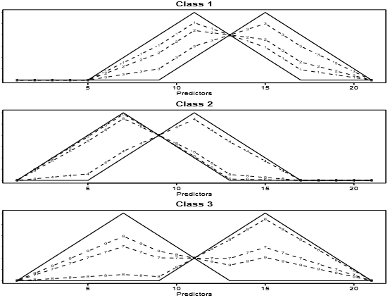 Figure 2: Some examples of the waveforms generated from model (46) before the Gaussian noise is added. The horizontal axis corresponds to the 21 predictor variables, and the vertical axis corresponds to the values of 21 predictor variables.加入高斯噪声之前由模型(46)产生的波形的一些例子。横轴对应21个预测变量,纵轴对应21个预测变量的值。
each method to have the same number of terminal nodes. This number is chosen via five-fold crossvalidation. We use an independent test sample of size 5000 to estimate the error rate. Averaged results over ten such independently drawn training-test set combinations are shown in Figure 3 and Table 1. As we can see, for this particular simulation example, SAMME performs slightly better than the AdaBoost.MH algorithm. A paired t-test across the ten independent comparisons indicates a significant difference with p-value around 0.003. We can also see that the SAMME.R algorithm performs closely to the SAMME algorithm.每个方法都有相同数量的终端节点。这个数字是通过5折交叉验证选择的。我们使用一个大小为5000的独立测试样本来估计错误率。十个独立抽样的训练-测试集组合的平均结果如图3和表1所示。我们可以看到,对于这个特定的模拟示例,SAMME的性能略优于AdaBoost.MH算法。10个独立组合比较的t检验表明有显著差异对应p值在0.003左右。也可看出SAMME.R和SAMME算法表现接近。
| Method | 200 Iterations | 400 | 600 |
|---|---|---|---|
| DT.CART | 28.4 (1.8) | ||
| Ada.MH | 17.1 (0.6) | 17.0 (0.5) | 17.0 (0.6) |
| SAMME | 16.7 (0.8) | 16.6 (0.7) | 16.6 (0.6) |
| SAMME.R | 16.8 (0.3) | 16.6 (0.4) | 16.6 (0.4) |
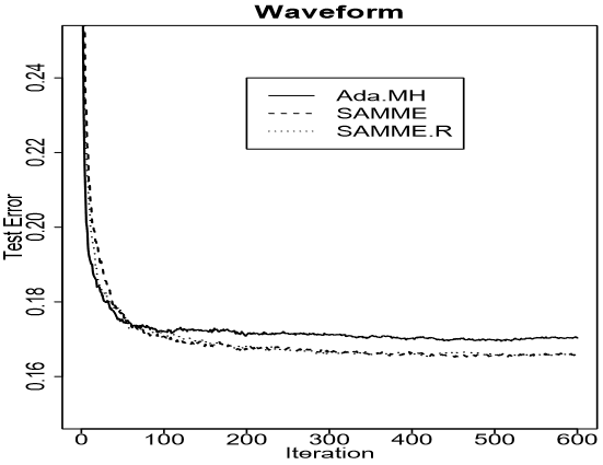 Figure 3: Test errors for SAMME, SAMME.R and AdaBoost.MH on the waveform simulation example. The training sample size is 300, and the testing sample size is 5000. The results are averages over ten independently drawn training-test set combinations.波形仿真实例的SAMME、SAMME.R和SAMME.R算法测试误差。训练样本量为300,测试样本量为5000。结果是平均自10个独立抽样的训练-测试集组合。
4.2 Real data实际数据
In this section, we show the results of running SAMME and SAMME.R on a collection of datasets from the UC-Irvine machine learning archive (Merz & Murphy 1998). Seven datasets were used: Letter, Nursery, Pendigits, Satimage, Segmentation, Thyroid and Vowel. These datasets come with pre-specified training and testing sets, and are summarized in Table 2. They cover a wide range of scenarios: the number of classes ranges from 3 to 26, and the size of the training data ranges from 210 to 16,000 data points. The types of input variables include both numerical and categorical, for example, in the Nursery dataset, all input variables are categorical variables. We used a classification tree as the weak classifier in each case. Again, the trees were built using a greedy, top-down recursive partitioning strategy. We restricted all trees within each method to have the same number of terminal nodes, and this number was chosen via five-fold cross-validation.在本节中,我们将展示运行SAMME和SAMME.R,这些数据集集合来自加州大学欧文分校机器学习档案(Merz & Murphy 1998)。所使用的七个数据集:Letter,Nursery,Pendigits,Satimage,Segmentation,Thyroid和Vowel。这些数据集带有预先指定的训练和测试集,总结在表2中。它们涵盖了广泛的场景:分类的数量从3到26个不等,培训数据的大小从210到16000个数据点不等。输入变量的类型包括数值变量和类别变量,例如在Nursery数据集中,所有输入变量都是类别变量。我们使用分类树作为每种情况下的弱分类器。同样,这些树是使用贪婪的、自顶向下递归的分区策略构建的。我们将每个方法中的所有树都限制为具有相同数量的终端节点,这个数量是通过5折交叉验证选择的。
Figure 4 compares SAMME and AdaBoost.MH. Since the SAMME.R algorithm performs closely to the SAMME algorithm, for exposition clarity, the test error curves for the SAMME.R algorithm are not shown. The test error rates are summarized in Table 4. The standard errors are approximated by $\sqrt{te.err·(1−te.err)/n.te}$, where $te.err$ is the test error, and $n.te$ is the size of the testing data.图4比较SAMME和AdaBoost.MH。由于SAMME.R算法的性能与SAMME算法非常接近,为了便于说明,没有显示SAMME.R算法的测试误差曲线。表4总结了测试错误率。误差标准差近似为$\sqrt{te.err·(1−te.err)/n.te}$,其中$te.err$为测试误差,$n.te$为测试数据的大小。
The most interesting result is on the Vowel dataset. This is a difficult classification problem, and the best methods achieve around 40% errors on the test data (Hastie, Tibshirani & Friedman 2001). The data was collected by Deterding (1989), who recorded examples of the eleven steady state vowels of English spoken by fifteen speakers for a speaker normalization study. The International Phonetic Association (IPA) symbols that represent the vowels and the words in which the eleven vowel sounds were recorded are given in the following table:最有趣的结果是Vowel数据集。这是一个很难分类的问题,最好的方法在测试数据上可以达到40%左右的误差(Hastie, Tibshirani & Friedman 2001)。这些数据是由Deterding(1989)收集的,他记录了15个说英语的人所说的11个稳定元音的例子,用于说话人的标准化研究。国际音标协会(IPA)下表列出了代表元音的符号以及记录了这11个元音的单词:
| Dataset | #Train | #Test | #Variables | #Classes |
|---|---|---|---|---|
| Letter | 16000 | 4000 | 16 | 26 |
| Nursery | 8840 | 3790 | 8 | 3 |
| Pendigits | 7494 | 3498 | 16 | 10 |
| Satimage | 4435 | 2000 | 36 | 6 |
| Segmentation | 210 | 2100 | 19 | 7 |
| Thyroid | 3772 | 3428 | 21 | 3 |
| Vowel | 528 | 462 | 10 | 11 |
| vowel | word | vowel | word | vowel | word | vowel | word |
|---|---|---|---|---|---|---|---|
| i: | heed | O | hod | I | hid | C: | hoard |
| E | head | U | hood | A | had | u: | who’d |
| a: | hard | 3: | heard | Y | hud |
Four male and four female speakers were used to train the classifier, and another four male and three female speakers were used for testing the performance. Each speaker yielded six frames of speech from eleven vowels. This gave 528 frames from the eight speakers used as the training data and 462 frames from the seven speakers used as the testing data. The ten predictors are derived from the digitized speech in a rather complicated way, but standard in the speech recognition world. As we can see from Figure 4 and Table 3, for this particular dataset, the SAMME algorithm performs almost 15% better than the AdaBoost.MH algorithm.使用4男4女说话者对分类器进行训练,使用4男3女说话者对分类器进行性能测试。每个说话者重复6遍这11个元音。这给了8个说话人528帧作为训练数据,来自7个说话人的462帧作为测试数据。这十个预测因子(特征变量)是由数字化语音以一种相当复杂的方式推导出来的,但在语音识别领域是标准的。从图4和表3可以看出,对于这个特定的数据集,SAMME算法的性能几乎比AdaBoost.MH算法好15%。
For other datasets, the SAMME algorithm performs slightly better than the AdaBoost.MH algorithm on Letter, Pendigits, and Thyroid, while slightly worse on Segmentation. In the Segmentation data, there are only 210 training data points, so the difference might be just due to randomness. It is also worth noting that for the Nursery data, both the SAMME algorithm and the AdaBoost.MH algorithm are able to reduce the test error to zero, while a single decision tree has about 0.8% test error rate. Overall, we are comfortable to say that the performance of SAMME is comparable with that of the AdaBoost.MH.在Letter、Pendigits和Thyroid数据集上,SAMME算法比AdaBoost.MH算法稍好,而在Segmentation数据集上则SAMME算法比AdaBoost.MH算法稍差。Segmentation只有210个训练样本,所以出现SAMME算法不如AdaBoost.MH算法可能是因为随机性。同样值得注意的是,对于Nursery数据,SAMME算法和AdaBoost.MH算法均能够将测试误差降至零,而单棵决策树的测试错误率约为0.8%。的来说,我们可以放心地说SAMME的性能不差于AdaBoost.MH。
For the purpose of further investigation, we also merged the training and the testing sets, and randomly split them into new training and testing sets. We then applied different methods on these new training and testing sets. The procedure was repeated ten times. The means of the test errors and the corresponding standard errors (in parentheses) are summarized in Table 5 and Figure 5. Again, the performance of SAMME is comparable with that of the AdaBoost.MH. We can see that for the Vowel data, the SAMME algorithm performs about 10% better than the AdaBoost.MH algorithm. A paired t-test across the ten independent comparisons indicates a significant difference with p-value around 0.001. For the Segmentation data, the test error rates are reversed: SAMME performs slightly better than AdaBoost.MH for this dataset. It is also interesting to note that the test error rate for the Pendigits data drops dramatically from 3% to about 0.6%. It turns out that in the original training-test split, the training digits were written by 30 writers, while the testing digits were written by 14 different writers. Unfortunately, who wrote which digits in the original data was not recorded. Therefore, in the re-split data, the 44 writers were mixed in both the training and testing data, which caused the drop in the test error rate.为了进一步的研究,我们还将训练集和测试集进行了合并,并将它们随机分为新的训练集和测试集。然后我们对这些新的训练和测试集应用了不同的方法。这个过程重复了十次。表5(遗憾这个表格没有见到)和图5总结了测试误差的均值和相应的误差标准差(括号内)。再次,SAMME的性能不差于AdaBoost.MH。可以看到,对Vowel数据,SAMME算法表现比AdaBoost.MH好10%。0个独立比较的配对t检验表明p值在0.001左右有显著差异。对于Segmentation数据,测试错误率颠倒过来(相对于原划分下的比较):SAMME的性能略优于AdaBoost.MH。有趣的是,Pendigits数据的测试错误率从3%急剧下降到0.6%左右。原来在原来的训练-测试分割中,训练数字是由30位作者编写的,而测试数字是由14位不同的作者编写的。不幸的是,谁写的哪些数字在原始数据中没有被记录。因此,在重新分割的数据中,训练数据和测试数据中混合了44位作者,导致了测试错误率的下降。
| Dataset | Method | 200 Iterations | 400 | 600 |
|---|---|---|---|---|
| Letter | DT.CART | 13.5 (0.5) | ||
| Ada.MH | 3.0 (0.3) | 2.8 (0.3) | 2.6 (0.3) | |
| SAMME | 2.6 (0.3) | 2.4 (0.2) | 2.3 (0.2) | |
| Nursery | DT.CART | 0.79 (0.14) | ||
| Ada.MH | 0 | 0 | 0 | |
| SAMME | 0 | 0 | 0 | |
| Pendigits | DT.CART | 8.3 (0.5) | ||
| Ada.MH | 3.0 (0.3) | 3.0 (0.3) | 2.8 (0.3) | |
| SAMME | 2.5 (0.3) | 2.5 (0.3) | 2.5 (0.3) | |
| Satimage | DT.CART | 13.8.4 (0.8) | ||
| Ada.MH | 8.7 (0.6) | 8.4 (0.6) | 8.5 (0.6) | |
| SAMME | 8.6 (0.6) | 8.2 (0.6) | 8.5 (0.6) | |
| Segmentation | DT.CART | 9.3 (0.6) | ||
| Ada.MH | 4.5 (0.5) | 4.5 (0.5) | 4.5 (0.5) | |
| SAMME | 4.9 (0.5) | 5.0 (0.5) | 5.1 (0.5) | |
| Thyroid | DT.CART | 0.64 (0.14) | ||
| Ada.MH | 0.67 (0.14) | 0.67 (0.14) | 0.67 (0.14) | |
| SAMME | 0.58 (0.13) | 0.61 (0.13) | 0.58 (0.13) | |
| Vowel | DT.CART | 53.0 (2.3) | ||
| Ada.MH | 52.8 (2.3) | 51.5 (2.3) | 51.5 (2.3) | |
| SAMME | 43.9 (2.3) | 43.3 (2.3) | 43.3 (2.3) |
 Figure 4: Test errors for SAMME and AdaBoost.MH on six benchmark datasets. These datasets come with pre-specified training and testing splits, and they are summarized in Table 2. The results for the Nursery data are not shown for the test error rates are reduced to zero for both methods. For exposition clarity, the results for SAMME.R are not shown because they are very close to SAMME.在6个基准数据集上测试SAMME和AdaBoost.MH的错误误差。这些数据集带有预先指定的训练和测试分支,表2总结了这些数据集。Nursery数据的结果没有显示,因为两种方法的测试错误率都降低到了零。为说明清楚,没有显示SAMME.R,因为它们与SAMME非常接近。
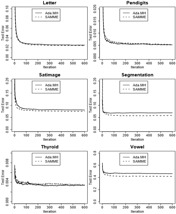 Figure 5: Test error for SAMME and AdaBoost.MH on six benchmark datasets. The results are averages over ten random training-test splits. The results for the Nursery data are not shown for the test error rates are reduced to zero for both methods. For exposition clarity, the results for SAMME.R are not shown because they are very close to SAMME.在6个基准数据集上测试SAMME和AdaBoost.MH的错误误差。结果平均自10次随机训练-测试集划分。Nursery数据的结果没有显示,因为两种方法的测试错误率都降低到了零。为说明清楚,没有显示SAMME.R,因为它们与SAMME非常接近。
5 Discussion讨论
The statistical view of boosting, as illustrated in Friedman et al. (2000), shows that the two-class AdaBoost builds an additive model to approximate the two-class Bayes rule. Following the same statistical principle, we have derived SAMME, the natural and clean multi-class extension of the two-class AdaBoost algorithm, and we have shown that Friedman等(2000)对boost的统计观点表明,两分类AdaBoost建立了一个叠加模型来近似两分类贝叶斯规则。根据同样的统计原理,我们推导出了SAMME,两分类AdaBoost算法的自然干净的多分类扩展,我们已经证明了
- SAMME adaptively implements the multi-class Bayes rule by fitting a forward stagewise additive model for multi-class problems;SAMME自适应地实现了多分类贝叶斯规则,它拟合了一个针对多分类问题的向前递归叠加模型;
- SAMME follows closely to the philosophy of boosting, i.e. adaptively combining weak classifiers (rather than regressors as in logit-boost (Friedman et al. 2000) and MART (Friedman 2001)) into a powerful one;SAMME紧跟boost的哲学,即自适应地将弱分类器(而不是logit-boost中的回归器 (Friedman et al. 2000)和MART (Friedman 2001))组合成强大的分类器;
- at each stage, SAMME returns only one weighted classifier (rather than
$K$), and the weak classifier only needs to be better than$K$-class random guessing;在每个阶段,SAMME只返回一个加权分类器(而不是$K$个),而弱分类器只需要比$K$类随机猜测更好; - SAMME shares the same simple modular structure of AdaBoost.SAMME采用了与AdaBoost相同的简单模块化结构。
We note that although AdaBoost was proposed to solve both the two-class and the multi-class problems (Freund & Schapire 1997), it sometimes can fail in the multi-class case. AdaBoost.MH is an approach to convert the $K$-class problem into $K$ two-class problems. As we have seen, AdaBoost.MH in general performs very well on both simulation and real-world data. SAMME’s performance is comparable with that of the AdaBoost.MH, and sometimes slightly better. However, we would like to emphasize that our goal is not to argue that SAMME is the ultimate multi-class classification tool, but rather to illustrate it is the natural extension of the AdaBoost algorithm to the multi-class case. We believe our numerical and theoretical results make SAMME an interesting and useful addition to the toolbox of multi-class methods. The SAMME algorithm has been implemented in the R computing environment, and will be publicly available from the first author’s website.我们注意到,虽然AdaBoost被提出来同时解决两分类和多分类问题(Freund & Schapire 1997),但它在多分类情况下有时会失败。AdaBoost.MH是一种将$K$类问题转换为$K$个两分类问题的方法。正如我们所看到的,AdaBoost.MH通常在模拟和真实数据上都表现得非常好。SAMME的性能与AdaBoost.MH相当,有时稍好一些。然而,我们想强调的是,我们的目标并不是证明SAMME是最终的多分类分类工具,而是说明它是AdaBoost算法对多分类情况的自然扩展。我们相信我们的数值和理论结果使SAMME成为多分类方法工具箱中一个有趣和有用的补充。SAMME算法已经在R计算环境中实现,并将在第一作者的网站上公开。
The multi-class exponential loss function (32) is a natural generalization of the two-class exponential loss function. Using the symmetry in $\vec{y}$ and $\vec{f}$, we can further simplify (32) as多分类指数损失函数(32)是两分类指数损失函数的自然推广。使用$\vec{y}$和$\vec{f}$的对称性,我们可以进一步简化(32)为
$$\exp \left(− \frac{1} {K −1} \sum_{k=1}^{K} \mathbb{I}(c = k)f_k\right)= \exp \left(− \frac{1} {K −1} f_c\right) \tag{47}$$
This naturally leads us to consider a general multi-class loss function that has the form:这自然会导致我们考虑具有这种形式的一般多分类损失函数:
$$\sum_{k=1}^{K} \mathbb{I}(c = k) \phi(f_k) \text{ or equivalently } \phi(f_c) \tag{48}$$
Hence, there are several interesting directions where our work can be extended: (8) For this general loss function to be sensible, we would like to find conditions on $\phi$ such that the classification rule given by the population minimizer agrees with the Bayes optimal rule. Lin (2004) studied a similar problem for the two-class classification case, and proposed very general conditions (Theorem 3.1). Along the lines of Lin (2004), we plan to design more multi-class loss functions that can be used in practice. (31) The principal attraction of the multi-class exponential loss function in the context of additive modeling is computational; it leads to our simple modular reweighting SAMME algorithm. We intend to develop algorithms for other members of the multi-class loss functions family as well.因此,有几个有趣的方向可以扩展我们的工作:(8)为了使这个一般的损失函数有意义,我们希望找到$\phi$的条件,使总体最小化给出的分类规则与贝叶斯最优规则一致。Lin(2004)研究了两分类分类情况下的一个类似问题,并提出了非常一般的条件(Theorem 3.1)。按照Lin(2004)的思路,我们计划设计更多可用于实践的多分类损失函数。(31)多分类指数损失函数在叠加建模中的主要吸引力是计算性的;这就引出了我们简单的模块化加权SAMME算法。我们还打算为多分类损失函数族的其他成员开发算法。
One example is the multi-class logit loss, which can be more robust to outliers and misspecified data. However, other multi-class loss functions may not lead to a simple closed form reweighting scheme. The computational trick used in Friedman (2001) and Buhlmann & Yu (2003) should prove useful here.个例子是多分类logit损失,它对异常值和具体错误的数据更加健壮。然而,其他多分类损失函数可能不会导致简单的封闭式重加权方案。Friedman(2001)和Buhlmann & Yu(2003)使用的计算技巧在这里应该是有用的。
Acknowledgments致谢
The authors would like to dedicate this work to the memory of Leo Breiman, who passed away while we were finalizing this manuscript. Leo Breiman has made tremendous contributions to the study of statistics and machine learning. His work has greatly influenced us. Zhu is partially supported by grant DMS-0505432 from the National Science Foundation. Hastie is partially supported by grant DMS-0204162 from the National Science Foundation.作者们想把这部作品献给Leo Breiman,他在我们完成手稿的时候去世了。Leo Breiman在统计学和机器学习方面做出了巨大的贡献。他的工作对我们影响很大。Zhu的研究得到了国家科学基金的部分资助。Hastie部分由国家科学基金会拨款DMS-0204162支持。
关于该选什么损失函数,参考6约10.5和10.6节有所介绍。
参考:
- 1.Y. Freund, and R. Schapire, “A Decision-Theoretic Generalization of On-Line Learning and an Application to Boosting”, 1997.;
- 2.J. Zhu, H. Zou, S. Rosset, T. Hastie. “Multi-class AdaBoost”, 2009.;
- 3.J. Zhu, S. Rosset, H. Zou, T. Hastie. “Multi-class AdaBoost”, 2005.;
- 4.H. Drucker. “Improving Regressors using Boosting Techniques”, 1997.;
- 5.David Pardoe and Peter Stone, “Boosting for Regression Transfer ”, 2010.;
- 6.T. Hastie, R. Tibshirani and J. Friedman, “Elements of Statistical Learning Ed. 2”, Springer, 2009.;
- 7.adaboost.M1与adaboost.M2差别比较;
- 8.sklearn文档1.11.3. AdaBoost ;
- 8.A Short Introduction to Boosting ;