feature engineering for machine mearning机器学习的特征工程alice zhang
1 The Machine Learning Pipeline机器学习管道
1.1 Data数据
What we call data are observations of real-world phenomena.对现实社会现象的观察称为数据。
1.2 Tasks任务
从数据到答案的道路就是任务。
1.3 Models模型
A mathematical model of data describes the relationships between different aspects of the data.数据的数学模型描述数据不同方面之间的关系。(数学模型说白了就是数学表达式。)
Mathematical formulas relate numeric quantities to each other. But raw data is often not numeric.数学表达式用数字联系彼此,但源数据不一定总是用数字表达的(可能用字符串等)。
1.4 Features特征
A feature is a numeric representation of raw data.特征是源数据的数字化表达。
some models are more appropriate for some types of features, and vice versa. The right features are relevant to the task at hand and should be easy for the model to ingest. Feature engineering is the process of formulating the most appropriate features given the data, the model, and the task. 特定模型有更适合的特征类型,当然特定特征类型也有更适合的模型。正确的特征与手头任务有关且应适合输入模型。生成最适合数据、模型、任务的特征的过程就是特征工程。
The number of features is also important. If there are not enough informative features, then the model will be unable to perform the ultimate task. If there are too many features, or if most of them are irrelevant, then the model will be more expensive and tricky to train.特征的数量也很重要。若无足够含信息的特征,模型将不能完成最终任务。若有太多特征,或特征大多(与任务)不相干,模型将更加难于训练。
1.5 Model Evaluation模型评估
Features and models sit between raw data and the desired insights. This is a double-jointed lever, and the choice of one affects the other. Good features make the subsequent modeling step easy and the resulting model more capable of completing the desired task.特征和模型位于源数据和目标洞察之间。这是一个双连接的杠杆,选择一个影响另一个。好的特性使后续的建模步骤更加容易,并且生成的模型更有能力完成目标任务。
2 Fancy Tricks with Simple Numbers简单数字的奇特技巧
统计数据类型分为互斥、穷尽的二分类数据、多分类数据、定序数据、二项式数据、计数、可加减实值数据、可乘除实值数据7类,前5类必定是离散数据、后两类可以是连续数据。详情见Statistical_data_type统计数据类型-我对wiki的翻译。
Good features should not only represent salient aspects of the data, but also conform to the assumptions of the model. Hence, transformations are often necessary. 好的特征不仅要表示数据的突出方面,而且要符合模型的假设。因此转换是必须的。
The first sanity check for numeric data is whether the magnitude matters.Do we just need to know whether it s positive or negative? Or perhaps we only need to know the magnitude at a very coarse granularity?对数字数据的首要的、明智的检查是大小是否重要。我们需要知道它是正的还是负的吗?或者我们只需要知道粒度非常粗的大小?
Next, consider the scale of the features. What are the largest and the smallest values? Do they span several orders of magnitude? Models that are smooth functions of input features are sensitive to the scale of the input. For example, $3x + 1$ is a simple linear function of the input x, and the scale of its output depends directly on the scale of the input. Other examples include k-means clustering, nearest neighbors methods, radial basis function (RBF) kernels, and anything that uses the Euclidean distance. For these models and modeling components, it is often a good idea to normalize the features so that the output stays on an expected scale.其次考虑数据的规模。最大和最小的值是多少?它们跨越几个数量级吗?输入特性平滑函数的模型对输入的规模很敏感。输入特性平滑函数的模型对输入的规模很敏感。例如$3x + 1$是输入$x$的一个简单线性方程,输出的规模直接决定于输入的规模。其他例子包括使用欧几里得距离的k-均值聚类、最近邻方法、径向基函数(RBF).对于这些模型或含有这些模型成分的模型,规范化特征以使之在期望的规模总是好的。
Logical functions, on the other hand, are not sensitive to input feature scale. Their output is binary no matter what the inputs are. For instance, the logical AND takes any two variables and outputs 1 if and only if both of the inputs are true. Another example of a logical function is the step function (e.g., is input x greater than 5?). Decision tree models consist of step functions of input features. Hence, models based on space-partitioning trees (decision trees, gradient boosted machines, random forests) are not sensitive to scale. The only exception is if the scale of the input grows over time, which is the case if the feature is an accumulated count of some sort—eventually it will grow outside of the range that the tree was trained on. If this might be the case, then it might be necessary to rescale the inputs periodically. Another solution is the bin-counting method.相反,逻辑函数不对输入特征的规模敏感。无论输入是什么,输出总是二元的。例如,逻辑“并”接受两个输入变量并得到输出1当且仅当两个输入变量为真。另一个例子是阶梯函数(如,$x$大于5吗?)。决策树模型由多个输入特征的阶梯函数组成。因此,基于空间划分树的模型(决策树、梯度提升机、随机森林)对规模不敏感。唯一的例外是,如果输入的规模随着时间的增长而增长(比方特性是某种累积计数),那么它最终将增长到树所训练的范围之外。如果是这样,那么就有必要定期重新调整输入。另一种解决方法是采用分箱计数的方法。(将在第5章介绍)
It’s also important to consider the distribution of numeric features. Distribution summarizes the probability of taking on a particular value. The distribution of input features matters to some models more than others. For instance, the training process of a linear regression model assumes that prediction errors are distributed like a Gaussian. This is usually fine, except when the prediction target spreads out over several orders of magnitude. In this case, the Gaussian error assumption likely no longer holds. One way to deal with this is to transform the output target in order to tame the magnitude of the growth. (Strictly speaking this would be target engineering, not feature engineering.) Log transforms, which are a type of power transform, take the distribution of the variable closer to Gaussian.考虑特征的分布也很重要。分布总结数据在某特定点的概率。模型是否受特征分布的影响,因模型而异。例如,线性回归模型的训练过程假设预测误差呈高斯分布。这种假设通常是合适的,除非预测目标跨越几个数量级。这种情况下,高斯误差假设无法成立。处理这种情况的一个方法是转换输出目标,为驯服数量级的增长。(严格讲,这将是目标工程而不是特征工程)对数转换,是一种幂变换,让变量的分布更接近高斯分布。
In addition to features tailoring to the assumptions of the model or training process, multiple features can be composed together into more complex features.Taken to an extreme, complex features may themselves be the output of statistical models. This is a concept known as model stacking.除了根据模型或训练过程的假设裁剪特性之外,多个特性还可以组合成更复杂的特性。如果走极端的话,复杂的特征本身可能就是统计模型的输出。这一概念叫模型堆叠。
Interaction features are simple to formulate, but the combination of features results in many more being input into the model. In order to reduce the computational expense, it is usually necessary to prune the input features using automatic feature selection. 交互特征容易计算,但模型组和导致模型中加入很多特征。为减少计算负担,通常需要使用自动特征选择来裁剪输入特征。
2.1 Scalars, Vectors, and Spaces标量、向量和空间
(略)
2.2 Dealing with Counts处理计数
In the age of Big Data, counts can quickly accumulate without bound. It is a good idea to check the scale and determine whether to keep the data as raw numbers, convert them into binary values to indicate presence, or bin them into coarser granularity. 大数据时代,计数极易无限制快速累积。检查(计数数据的)规模并决定是否保持源数据,是否转换成表示存在性的二元值,是否按粗略粒度将之分箱是一个好主意。
可不可以对计数counting进行scaling等,难道只可以二值化或分箱吗?是否该处理的依据是什么?采用哪种处理的一句是什么?是不是因为计数是离散型数据所以不可以scaling等这样会变成小数?因该是因为这个!二值化或分箱后的数据仍然是离散型,必须保证这些离散特征符合任务等的要求,可能就是因该根据这选择合适处理方法。
2.2.1 Binarization二值化
计数的二值化是计数的鲁棒性表示(即为了鲁棒性)。作者并未讲什么时候该进行计数的二值化,为什么是二值化而不是量化或分箱。“这样,模型将不必费力去预测原始计数的时间差异”,可能按作者意思,是否对计数进行处理,作何处理,取决于任务(精度要求)。
2.2.2 Quantization or Binning量化或分箱
Raw counts that span several orders of magnitude are problematic for many models. In a linear model, the same linear coefficient would have to work for all possible values of the count. Large counts could also wreak havoc in unsupervised learning methods such as k-means clustering, which uses Euclidean distance as a similarity function to measure the similarity between data points. A large count in one element of the data vector would outweigh the similarity in all other elements, which could throw off the entire similarity measurement.对于许多模型来说,跨越几个数量级的原始计数是有问题的。在线性模型中,相同的线性系数对计数的所有可能值都应成立。大量的计数也会对k-means聚类等非监督学习方法造成破坏,k-means聚类利用欧氏距离作为相似性函数来度量数据点之间的相似性。数据向量中一个元素的数值很大的计数对相似度的贡献超过其他元素,这可能会影响整个相似性度量。
One solution is to contain the scale by quantizing the count. In other words, we group the counts into bins, and get rid of the actual count values. Quantization maps a continuous number to a discrete one. We can think of the discretized numbers as an ordered sequence of bins that represent a measure of intensity.一种解决方案是通过量化计数来控制规模。换句话说,我们将计数分组到容器中,并去掉实际的计数值。量化把一个连续的数映射为一个离散的数。我们可以把离散的数字看作是一组有序的箱子,代表着强度的度量。
In order to quantize data, we have to decide how wide each bin should be. The solutions fall into two categories: fixed-width or adaptive.为了量化数据,我们必须决定每个箱子的宽度。解决方案分为两类:固定宽度或自适应。
2.2.2.1 Fixed-width binning
With fixed-width binning, each bin contains a specific numeric range. The ranges can be custom designed or automatically segmented, and they can be linearly scaled or exponentially scaled. When the numbers span multiple magnitudes, it may be better to group by powers of 10 (or powers of any constant). Exponential-width binning is very much related to the log transform. 对于固定宽度的箱,每个箱包含一个特定的数值范围。范围可以自己设计或自动分割,它们可以线性缩放或指数缩放。当这些数字跨越多个量级时,最好以10的乘方(或任何常数的乘方)进行分组。指数宽度分箱与对数变换有很大关系。(将在2.3节介绍)
2.2.2.2 Quantile binning
Fixed-width binning is easy to compute. But if there are large gaps in the counts, then there will be many empty bins with no data. This problem can be solved by adaptively positioning the bins based on the distribution of the data. This can be done using the quantiles of the distribution.固定宽度的装箱很容易计算。但是如果计数有很大的差距,那么就会有很多没有数据的空箱子。这个问题可以通过根据数据的分布来自适应地定位容器来解决。可以用分布的分位数来实现。
Quantiles are values that divide the data into equal portions. 分位数是将数据分成相等部分的值。
2.3 Log Transformation对数变换
In other words, the log function compresses the range of large numbers and expands the range of small numbers. The larger x is, the slower log(x) increments.换句话说,log函数压缩了大数的范围,扩展了小数的范围。x越大,log(x)增量越慢。
The log transform is a powerful tool for dealing with positive numbers with a heavy-tailed distribution. (A heavy-tailed distribution places more probability mass in the tail range than a Gaussian distribution.) It compresses the long tail in the high end of the distribution into a shorter tail, and expands the low end into a longer head. 对数变换是处理带有重尾分布的正数的强大工具。(重尾分布比高斯分布的概率质量更大。)它将分布高值端的长尾巴压缩成较短的尾巴,并将低值端的尾巴展开成较长的头部。
2.3.1 Log Transformation in Action对数变换实操
2.3.2 Power Transforms: Generalization of the Log Transform幂变换:对数变换的泛化
The log transform is a specific example of a family of transformations known as power transforms. In statistical terms, these are variance-stabilizing transformations.对数转换是称为幂转换的一系列转换的一个特定示例。从统计学的角度来看,这些是稳定变量的转换。
The Box-Cox formulation only works when the data is positive. For nonpositive data, one could shift the values by adding a fixed constant. When applying the Box-Cox transformation or a more general power transform, we have to determine a value for the parameter $\lambda$. This may be done via maximum likelihood (finding the λ that maximizes the Gaussian likelihood of the resulting transformed signal) or Bayesian methods. Box-Cox公式只有在数据为正数时才有效。对于非正数据,可以通过添加一个固定常数来改变值。应用Box-Cox时转换或更一般的电力变换,我们必须确定参数$\lambda$的值。这可通过最大似然(发现使结果转换信号的高斯似然最大的$\lambda$)或贝叶斯方法得到。
A probability plot, or probplot, is an easy way to visually compare an empirical distribution of data against a theoretical distribution. This is essentially a scatter plot of observed versus theoretical quantiles. 概率图是一种简单的方法,可以直观地将数据的经验分布与理论分布进行比较。这本质上是观测量和理论量的散点图。
2.4 Feature Scaling or Normalization特征缩放或规范化
Models that are smooth functions of the input, such as linear regression, logistic regression, or anything that involves a matrix, are affected by the scale of the input. Tree-based models, on the other hand, couldn’t care less. If your model is sensitive to the scale of input features, feature scaling could help. As the name suggests, feature scaling changes the scale of the feature. Sometimes people also call it feature normalization. Feature scaling is usually done individually to each feature.输入平滑函数的模型,如线性回归、逻辑回归或任何涉及矩阵的模型,都会受到输入规模的影响。另一方面,基于树的模型却毫不在意输入规模。如果您的模型对输入特性的规模很敏感,那么特性缩放可能会有帮助。顾名思义,特性缩放改变了特性的大小。有时人们也称它为特性规范化。特性缩放通常是对每个特性单独进行的。
2.4.1 Min-Max Scaling 最小-最大值缩放
Min-max scaling squeezes (or stretches) all feature values to be within the range of [0, 1]. 最小-最大值缩放挤压(或拉伸)所有特征值都在[0,1]的范围内。
2.4.2 Standardization (Variance Scaling) 标准化(方差缩放)
It subtracts off the mean of the feature (over all data points) and divides by the variance. Hence, it can also be called variance scaling. The resulting scaled feature has a mean of 0 and a variance of 1. If the original feature has a Gaussian distribution, then the scaled feature does too.它减去特征的平均值(除以所有数据点),然后除以方差。因此,它也可以称为方差缩放。缩放特征结果的平均值为0,方差为1。如果原始特征具有高斯分布,则缩放特征也具有高斯分布。
Use caution when performing min-max scaling and standardization on sparse features. If the shift is not zero, then these two transforms can turn a sparse feature vector where most values are zero into a dense one.在稀疏特性上执行最小最大缩放和标准化时要小心。如果位移不为零,那么这两个变换就可以将大多数值为零的稀疏特征向量变为稠密特征向量。
2.4.3 ℓ2 Normalization ℓ2规范化
This technique normalizes (divides) the original feature value by what’s known as the $ℓ^2$ norm, also known as the Euclidean norm. The $ℓ^2$ norm measures the length of the vector in coordinate space. The $ℓ^2$ norm sums the squares of the values of the features across data points, then takes the square root. After ℓ2 normalization, the feature column has norm 1. This is also sometimes called $ℓ^2$ scaling. (Loosely speaking, scaling means multiplying by a constant, whereas normalization could involve a number of operations.)这种技术将原始特征值用所谓的$ℓ^2$范数(也称为欧几里德范数)来标准化(分割)。$ℓ^2$范数测量的是坐标空间中向量的长度。$ℓ^2$范数对数据点上特征值的平方求和,然后取平方根。特征列具有范数1。这有时也称为$ℓ^2$缩放。(宽松地说,缩放意味着乘以一个常数,而规范化可能涉及到许多操作。)
unlike the log transform, feature scaling doesn’t change the shape of the distribution; only the scale of the data changes.与对数变换不同,特征缩放不会改变分布的形状;只有数据的规模发生了变化。
Feature scaling is useful in situations where a set of input features differs wildly in scale. Drastically varying scale in input features can lead to numeric stability issues for the model training algorithm. In those situations, it’s a good idea to standardize the features.在一组输入特性在规模上相差很大的情况下,特性缩放是很有用的。剧烈的规模差异会导致模型训练算法的数值稳定性问题。在这种情况下,标准化特性是一个好主意。
2.5 Interaction Features交互特征
generalized linear models often find interaction features very helpful.交互特征在广义线性模型经常非常有用。
Interaction features are very simple to formulate, but they are expensive to use. The training and scoring time of a linear model with pairwise interaction features would go from $O(n)$ to $O(n^2)$, where $n$ is the number of singleton features.交互特征非常简单,但是使用起来很昂贵。含有两两交互特征的线性模型训练和评分时间将从$O(n)$升到$O(n^2)$,其中$n$是特征数量。
There are a few ways around the computational expense of higher-order interaction features. One could perform feature selection on top of all of the interaction features. 关于高阶交互特性的计算开销有几种方法。可以在所有交互特性之上执行特征选择。
Alternatively, one could more carefully craft a smaller number of complex features.或者,可以更仔细地设计以减少复杂特征数量。
Both strategies have their advantages and disadvantages. Feature selection employs computational means to select the best features for a problem. (This technique is not limited to interaction features.) However, some feature selection techniques still require training multiple models with a large number of features.这两种策略各有利弊。特征选择使用计算方法为问题选择最佳特征。(这种技术并不局限于交互特性。)然而,一些特征选择技术仍然需要训练具有大量特征的多个模型。
Handcrafted complex features can be expressive enough that only a small number of them are needed, which reduces the training time of the model—but the features themselves may be expensive to compute, which increases the computational cost of the model scoring stage. 手工制作的复杂特性的表达能力非常强,只需要少量的特性,这减少了模型的训练时间,但是特性本身的计算成本可能很高,这增加了模型评分阶段的计算成本。
2.6 Feature selection特征选择
Feature selection techniques prune away nonuseful features in order to reduce the complexity of the resulting model. The end goal is a parsimonious model that is quicker to compute, with little or no degradation in predictive accuracy. 特征选择技术删除无用的特征,以减少结果模型的复杂性。最终目标是一个简洁的模型,计算速度更快,预测准确率几乎没有下降。
Roughly speaking, feature selection techniques fall into three classes:粗略地说,特性选择技术分为三类:
Filtering过滤
Filtering techniques preprocess features to remove ones that are unlikely to be useful for the model. Filtering techniques are much cheaper than the wrapper techniques, but they do not take into account the model being employed. Hence, they may not be able to select the right features for the model.过滤技术对特征进行预处理,以去除那些对模型不太有用的特征。过滤技术比包装技术便宜得多,但它们没有考虑所使用的模型。因此,他们可能无法为模型选择最正确的特性。
Wrapper methods包装方法
These techniques are expensive, but they allow you to try out subsets of features, which means you won’t accidentally prune away features that are uninformative by themselves but useful when taken in combination. 这些技术是昂贵的,但它们允许您尝试特性的子集,这意味着您不会意外地删除那些本身不提供信息但结合使用时有用的特性。
Embedded methods嵌入式方法
These methods perform feature selection as part of the model training process. Embedded methods incorporate feature selection as part of the model training process. They are not as powerful as wrapper methods, but they are nowhere near as expensive. Compared to filtering, embedded methods select features that are specific to the model. In this sense, embedded methods strike a balance between computational expense and quality of results.这些方法作为模型训练过程的一部分来执行特征选择。嵌入式方法将特征选择作为模型训练过程的一部分。它们没有包装器方法那么强大,但是它们远没有包装器那么昂贵。与过滤相比,嵌入式方法选择特定于模型的特性。从这个意义上说,嵌入式方法在计算开销和结果质量之间取得了平衡。
2.7 Summary总结
2.8 Bibliography文献目录
3 Text Data: Flattening, Filtering, and Chunking文本数据:扁平化、过滤和分块
暂时不是我的兴趣点,有空再学
3.1 Bag-of-X: Turning Natural Text into Flat Vectors x袋模型:将自然文本转化为扁平向量
3.1.1 Bag-of-Words词袋模型
3.1.2 Bag-of-n-Grams n-Grams袋模型
3.2 Filtering for Cleaner Features过滤以得到更干净特征
3.2.1 Stopwords停止词
3.2.2 Frequency-Based Filtering 基于频率的过滤
3.2.3 Stemming字干搜寻
3.3 Atoms of Meaning: From Words to n-Grams to Phrases意义的原子:从词到n-Grams再到短语
3.3.1 Parsing and Tokenization解析和标记
3.3.2 Collocation Extraction for Phrase Detection为短语检测搭配提取
3.4 Summary总结
3.5 Bibliography文献目录
4 The Effects of Feature Scaling: From Bag-of-Words to Tf-Idf特征缩放的效果:从词袋到Tf-Idf
暂时不是我的兴趣点,有空再学
4.1 Tf-Idf : A Simple Twist on Bag-of-WordsTf-Idf:词袋的一个简单变形
4.2 Putting It to the Test让它接受考验
4.2.1 Creating a Classification Dataset创建分类数据集
4.2.2 Scaling Bag-of-Words with Tf-Idf Transformation用Tf-Idf转换缩放词袋模型
4.2.3 Classification with Logistic Regression用逻辑回归模型分类
4.2.4 Tuning Logistic Regression with Regularization用正则化调整逻辑回归
4.3 Deep Dive: What Is Happening?深度理解:发生了什么?
4.4 Summary总结
4.5 Bibliography文献目录
5 Categorical Variables: Counting Eggs in the Age of Robotic Chickens分类变量:机器鸡时代的鸡蛋计数
A categorical variable, as the name suggests, is used to represent categories or labels. The number of category values is always finite in a real-world dataset. The values may be represented numerically. However, unlike other numeric variables, the values of a categorical variable cannot be ordered with respect to one another. They are called nonordinal.顾名思义,类别变量用于表示类别或标签。在实际数据集中,类别值的数量总是有限的。这些值可以用数字表示。然而,与其他数值变量不同的是,类别变量的值不能相互排序。它们被称为非序数。
注意:分类变量categorical variable是一种离散变量discrete variable,离散变量是分类变量的超集,两者并不完全等价。因为离散变量不一定非序数nonordinal,例如计数counting当然是离散的,但绝不是非序数nonordinal。
5.1 Encoding Categorical Variables编码分类变量
The categories of a categorical variable are usually not numeric. Thus, an encoding method is needed to turn these nonnumeric categories into numbers. It is tempting to simply assign an integer, say from 1 to k, to each of k possible categories—but the resulting values would be orderable against each other, which should not be permissible for categories. 分类变量的类别通常不是数字。因此,需要一种编码方法将这些非数字类别转换为数字。尝试简单地将一个整数(比如从1到k)赋给k个可能的类别中的每一个,但是结果值是可以相互排序的,这对于类别来说是不允许的。
5.1.1 One-Hot Encoding独热编码
A better method is to use a group of bits. Each bit represents a possible category. If the variable cannot belong to multiple categories at once, then only one bit in the group can be “on.” This is called one-hot encoding.更好的方法是使用一组位。每个位代表一个可能的类别。如果变量不能同时属于多个类别,那么组中只能有一个位可用。这被称为独热编码。
One-hot encoding is very simple to understand, but it uses one more bit than is strictly necessary. If we see that $k–1$ of the bits are 0, then the last bit must be 1 because the variable must take on one of the $k$ values. Mathematically, one can write this constraint as “the sum of all bits must be equal to 1”:独热编码非常容易理解,但是它使用的位比严格需要的多一位。如果我们看到前$k-1$位都是0,那么最后一个位必须是1,因为变量必取1到$k$中的一个值。从数学上讲,可以把这个约束写成所有位的和一定等于1: $$e_1 + e_2 + \dots + e_k = 1$$ Thus, we have a linear dependency on our hands. Linear dependent features, as we discovered in Chapter 4, are slightly annoying because they mean that the trained linear models will not be unique. Different linear combinations of the features can make the same predictions, so we would need to jump through extra hoops to understand the effect of a feature on the prediction.因此,目前是线性依赖的。线性相关的特征,第四章讨论过,有点恼人,因为它们意味着训练过的线性模型不会是唯一的。不同特征的线性组合可以做出相同的预测,因此我们需要跳过额外的障碍来理解特征对预测的影响。
5.1.2 Dummy Coding哑编码
The problem with one-hot encoding is that it allows for $k$ degrees of freedom, while the variable itself needs only $k-1$. Dummy coding removes the extra degree of freedom by using only $k-1$ features in the representation. One feature is thrown under the bus and represented by the vector of all zeros. This is known as the reference category. 独热编码的问题是它允许$k$个自由度,而变量本身只需要$k-1$个。哑编码通过在表示中只使用$k-1$特性来消除额外的自由度。一个特性被丢到总线下,由全含0的向量表示。全零向量就是所谓参考分类。
With one-hot encoding, the intercept term represents the global mean of the target variable, and each of the linear coefficients represents how much that target variable differs from the global mean.采用独热编码,截距代表目标变量的全局均值,每个线性系数表示目标变量与全局均值的差值。
With dummy coding, the bias coefficient represents the mean value of the response variable y for the reference category. The coefficient for the ith feature is equal to the difference between the mean response value for the ith category and the mean of the reference category.通过哑编码,偏置系数表示参考类别响应变量y的均值。第i个特征的系数等于第i个类别的平均响应值与参考类别的平均响应值之差。
5.1.3 Effect Coding效果编码
Yet another variant of categorical variable encoding is effect coding. Effect coding is very similar to dummy coding, with the difference that the reference category is now represented by the vector of all –1’s.分类变量编码的另一种变体是效果编码。效果编码与哑编码非常相似,不同的是,参考类别现在由全是-1值的向量表示。
Effect coding is very similar to dummy coding, but results in linear regression models that are even simpler to interpret. The intercept term represents the global mean of the target variable, and the individual coefficients indicate how much the means of the individual categories differ from the global mean. (This is called the main effect of the category or level, hence the name “effect coding.”) One-hot encoding actually came up with the same intercept and coefficients, but in that case there are linear coefficients for each category. 效果编码与哑编码非常相似,但结果是线性回归模型,解释起来更加简单。截距项表示目标变量的全局均值,单个系数表示各个类别的均值与全局均值的差值。(这称为类别或级别的主效果,因此称为名称效果编码。)独热编码实际上得到了相同的截距和系数,但在这种情况下,每个分类都有线性系数。
5.1.4 Pros and Cons of Categorical Variable Encodings分类变量编码的利弊
One-hot, dummy, and effect coding are very similar to one another. They each have pros and cons. One-hot encoding is redundant, which allows for multiple valid models for the same problem. The nonuniqueness is sometimes problematic for interpretation, but the advantage is that each feature clearly corresponds to a category. Moreover, missing data can be encoded as the all-zeros vector, and the output should be the overall mean of the target variable.独热编码、哑编码和效果编码很相似。均有利弊。独热编码是冗余的,这允许对同一个问题使用多个有效模型。非唯一性对于解释来说有时是有问题的,但其优点是每个特性都明显对应于一个类别。而且,缺失数据可以编码为全零向量,输出为目标变量的总体均值。
Dummy coding and effect coding are not redundant. They give rise to unique and interpretable models. The downside of dummy coding is that it cannot easily handle missing data, since the all-zeros vector is already mapped to the reference category. It also encodes the effect of each category relative to the reference category, which may look strange.哑编码和效果编码不存在冗余。它们产生了独特的、可解释的模型。哑编码的缺点是它不能轻易地处理丢失的数据,因为全零向量已经映射到引用类别。它还对每个类别相对于参考类别的效果进行编码,这看起来可能很奇怪。
Effect coding avoids this problem by using a different code for the reference category, but the vector of all –1’s is a dense vector, which is expensive for both storage and computation. For this reason, popular ML software packages such as Pandas and scikit-learn have opted for dummy coding or one-hot encoding instead of effect coding.效果编码通过为参考类别使用不同的向量来避免了这个问题,但值全为-1的参考类别是一个密集的向量,对于存储和计算来说都是昂贵的。
All three encoding techniques break down when the number of categories becomes very large. Different strategies are needed to handle extremely large categorical variables. 当类别数量变得非常大时,所有这三种编码技术都会崩溃。处理非常大的分类变量需要不同的策略。
5.2 Dealing with Large Categorical Variables处理大的分类变量
Existing solutions can be categorized (haha) thus:现有的解决方案可以这样分类:
- Do nothing fancy with the encoding. Use a simple model that is cheap to train. Feed one-hot encoding into a linear model (logistic regression or linear support vector machine) on lots of machines.对编码不做任何花哨的处理。使用一个便宜的简单模型来训练。在许多机器上(我理解on lots of machines是指在很多机器学习问题上),将一个热编码输入一个线性模型(逻辑回归或线性支持向量机)。
- Compress the features. There are two choices: 压缩特征,有两个选择:特征哈希,线性模型常用;分箱计数,线性模型和基于树的模型均常用。 2.1. Feature hashing, popular with linear models 2.2. Bin counting, popular with linear models as well as trees
注意:Large Categorical Variables切不可与混淆rare categories混淆。Large Categorical Variables是指含有很多分类,即分类的数量很多,各个分类的数据点数量可能平衡也可能不平衡;rare categories是指一些分类在数据点中很少出现,也即各个分类所含的点的数量很不平衡,分类的数量很可能很多,但也可能不多。
5.2.1 Feature Hashing特征哈希
A hash function is a deterministic function that maps a potentially unbounded integer to a finite integer range [1, m]. Since the input domain is potentially larger than the output range, multiple numbers may get mapped to the same output. This is called a collision. A uniform hash function ensures that roughly the same number of numbers are mapped into each of the m bins.哈希函数是一个确定性函数,它将一个潜在的无界整数映射到一个有限整数范围[1,m]。既然输入域可能大于输出范围,因此多个数字可能映射到相同的输出。这叫做冲突。一个均匀的哈希函数确保m个容器中每个容器映射得到大致相同数量的数字。
Hash functions can be constructed for any object that can be represented numerically (which is true for any data that can be stored on a computer): numbers, strings, complex structures, etc.任何对象(对于可存储于计算机的任何数据),诸如数字、字符串、复杂结构等,均可通过哈希函数将之数字化表示。
我的理解是先哈希到[1,m]整数范围,再执行独热编码/哑编码/效果编码
For instance, if the original features were words in a document, then the hashed version would have a fixed vocabulary size of m, no matter how many unique words there are in the input. 例如,如果原始特性是文档中的单词,那么哈希版本的词汇表大小将固定为m,而不管输入中有多少独特单词。
Another variation of feature hashing adds a sign component, so that counts are either added to or subtracted from the hashed bin. Statistically speaking, this ensures that the inner products between hashed features are equal in expectation to those of the original features.特性哈希的另一个变体添加了一个正负符号组件,因此计数可以从哈希存储中添加或减去(等可能,比如奇数时候用减号偶数用加号)。从统计学上讲,这确保了哈希后的特征之间的内积与原始特征在期望上是相等的。
The value of the inner product after hashing is within O(1/m) of the original inner product, so the size of the hash table m can be selected based on acceptable errors. In practice, picking the right m could take some trial and error.哈希后的内积的值在原始内积的O(1/m)内,因此可以根据可接受的错误选择哈希表m的大小。在实践中,选择正确的m可能需要一些尝试并承受一些错误。
Feature hashing can be used for models that involve the inner product of feature vectors and coefficients, such as linear models and kernel methods. It has been demonstrated to be successful in the task of spam filtering.特征哈希可以用于包含特征向量和系数内积的模型,如线性模型和核方法。实践证明,该方法在垃圾邮件过滤方面是成功的。
One downside to feature hashing is that the hashed features, being aggregates of original features, are no longer interpretable.特征哈希的一个缺点是,哈希后的特征是原始特征的聚合,不再是可解释的。
5.2.2 Bin Counting分箱计数
The idea of bin counting is deviously simple: rather than using the value of the categorical variable as the feature, instead use the conditional probability of the target under that value. In other words, instead of encoding the identity of the categorical value, we compute the association statistics between that value and the target that we wish to predict. For those familiar with naive Bayes classifiers, this statistic should ring a bell, because it is the conditional probability of the class under the assumption that all features are independent.分箱计算的思想非常简单:(在分类数量太多时候),与其使用分类变量的值作为特性,不如使用该值下目标的条件概率。换句话说,我们不是编码分类值的标识,而是计算该值与我们希望预测的目标之间的关联统计信息。对于那些熟悉朴素贝叶斯分类器的人来说,这个统计量应该会让人想起,因为它是在假设所有特征都是独立的前提下,一个分类的条件概率。
| Users | Number of clicks | Number of nonclicks | Probability of clicks | QueryHash, AdDomain | Number of clicks | Number of nonclicks | Probability of click |
|---|---|---|---|---|---|---|---|
| Alice | 5 | 120 | 0.0400 | 0x598fd4fe, foo.com | 5,000 | 30,000 | 0.167 |
| Bob | 20 | 230 | 0.0800 | 0x50fa3cc0, bar.org | 100 | 900 | 0.100 |
| … | … | ||||||
| Joe | 2 | 3 | 0.400 | 0x437a45e1, qux.net | 6 | 18 | 0.250 |
Bin counting assumes that historical data is available for computing the statistics. Table 5-6 contains aggregated historical counts for each possible value of the categorical variables. Based on the number of times the user “Alice” has clicked on any ad and the number of times she has not clicked, we can calculate the probability of her clicking on any ad. Similarly, we can compute the probability of a click for any query–ad domain combination. At training time, every time we see “Alice,” we can use her probability of click as the input feature to the model. The same goes for QueryHash–AdDomain pairs like “0x437a45e1, qux.net.”分箱计算假设历史数据可以用于计算统计数据。表5-6包含分类变量的每个可能值的汇总历史计数。根据用户Alice点击任何广告的次数和她没有点击的次数,我们可以计算她点击任何广告的概率。类似地,我们可以计算任何查询广告域组合的点击概率。在训练时,每次我们看到Alice,我们都可以用她的点击概率作为模型的输入特征。对“QueryHash, AdDomain”特征也一样,比如“0x437a45e1,qux.net”。
Suppose there were 10,000 users. One-hot encoding would generate a sparse vector of length 10,000, with a single 1 in the column that corresponds to the value of the current data point. Bin counting would encode all 10,000 binary columns as a single feature with a real value between 0 and 1.假设有10,000用户。独热编码将生成长度为10,000的稀疏向量,列中的单个1对应于当前数据点的值。分箱计算将所有10,000个二进制列编码为一个特性,其实际值介于0和1之间。
We can include other features in addition to the historical click-through probability: the raw counts themselves (number of clicks and nonclicks), the log-odds ratio, or any other derivatives of probability. Our example here is for predicting ad click-through rates, but the technique readily applies to general binary classification. It can also be readily extended to multiclass classification using the usual techniques to extend binary classifiers to multiclass; i.e., via one-against-many odds ratios or other multiclass label encodings.除了历史点击通过概率之外,我们还可以包含其他特性:原始计数本身(点击次数和非点击次数)、对数优势比,或概率的任何其他衍生物。我们这里的示例用于预测广告点击率,但该技术很容易应用于一般的二元分类。它还可以很容易地扩展到多类分类,使用通常的技术将二进制分类器扩展到多类;如通过一对多优势或其他多类标签编码。
In short, bin counting converts a categorical variable into statistics about the value. It turns a large, sparse, binary representation of the categorical variable, such as that produced by one-hot encoding, into a very small, dense, real-valued numeric representation.简而言之,分箱计算将分类变量转换为关于值的统计值。它将分类变量的一个大的、稀疏的、二进制的表示,例如由独热编码产生的,变成一个非常小的、密集的、实值的数值表示。
In terms of implementation, bin counting requires storing a map between each category and its associated counts. (The rest of the statistics can be derived on the fly from the raw counts.) Hence it requires O(k) space, where k is the number of unique values of the categorical variable.说到实现方法,分箱计算需要存储分类到关联计算值的映射。(其余的统计数据可以从原始数据中动态地得到。)因此,它需要O(k)维空间,其中k是类别变量的独特值的数量。
What about rare categories?罕见分类怎么办?
Just like rare words, rare categories require special treatment. Think about a user who logs in once a year: there will be very little data to reliably estimate that user’s click-through rate for ads. Moreover, rare categories waste space in the counts table.就像罕见的词语一样,罕见的类别也需要特殊的处理。想想每年登录一次的用户:只有很少的数据可以可靠地估计用户的广告点击率。此外,罕见分类浪费了计数表中的空间。
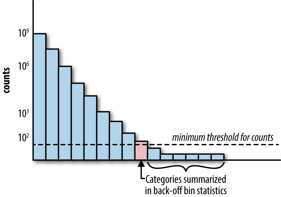
One way to deal with this is through back-off, a simple technique that accumulates the counts of all rare categories in a special bin (see Figure 5-3). If the count is greater than a certain threshold, then the category gets its own count statistics. Otherwise, we use the statistics from the back-off bin. This essentially reverts the statistics for a single rare category to the statistics computed on all rare categories. When using the back-off method, it helps to also add a binary indicator for whether or not the statistics come from the back-off bin.处理这个问题的一种方法是通过back-off,这是一种简单的技术,可以在一个特殊的容器中累积所有稀有类别的计数(参见图5-3)。如果计数大于某个阈值,则类别将获得自己的计数统计信息。否则,我们将使用back-off容器中的统计数据。这实际上是将单个罕见类别的统计信息还原为所有罕见类别的统计信息。在使用back-off方法时,还可以添加一个二进制指示器,以指示统计数据是否来自back-off容器。
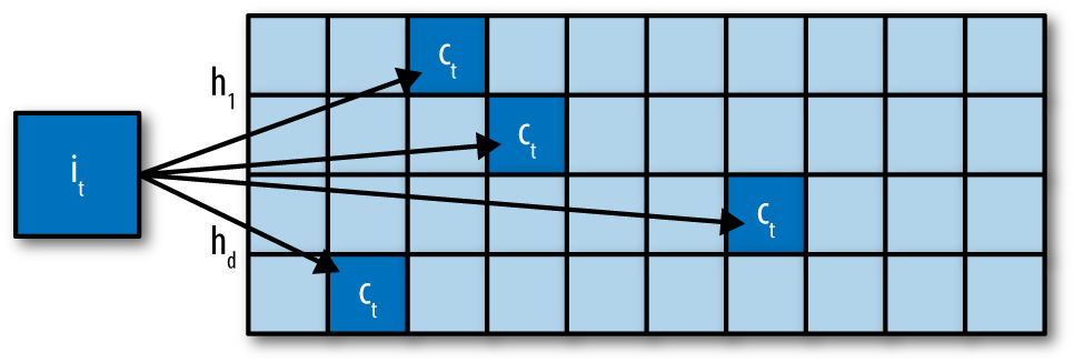
There is another way to deal with this problem, called the count-min sketch (Cormode and Muthukrishnan, 2005). In this method, all the categories, rare or frequent alike, are mapped through multiple hash functions with an output range, m, much smaller than the number of categories, k. When retrieving a statistic, recompute all the hashes of the category and return the smallest statistic. Having multiple hash functions mitigates the probability of collision within a single hash function. The scheme works because the number of hash functions times m, the size of the hash table, can be made smaller than k, the number of categories, and still retain low overall collision probability.还有另一种方法来处理这个问题,叫做“数分钟素描”count-min sketch(Cormode和Muthukrishnan, 2005)。在这种方法中,所有的类别,无论是罕见的还是频繁的,都是通过哈希函数映射到输出范围为m的多个值,其输出范围远小于类别的数量k。在检索统计信息时,重新计算类别的所有散列并返回最小的统计信息。该方案之所以有效,是因为哈希函数的数量乘以哈希表的大小m,可以使其小于类别的数量k,并且仍然保持较低的总体冲突概率。
Figure 5-4 illustrates. Each item i is mapped to one cell in each row of the array of counts. When an update of $c_t$ to item $i_t$ arrives, $c_t$ is added to each of these cells, hashed using functions $h_1…h_d$.图5-4揭示每个项i映射到计数数组的每行中的一个单元格。当$c_t$的更新对项目$i_t$到来时,$c_t$会被添加到这些单元中,使用$h_1$到$h_d$函数进行散列。
这个count-min sketch我还是没搞懂在扯什么淡,有空再了解吧
Guarding against data leakage防止数据泄漏
Since bin counting relies on historical data to generate the necessary statistics, it requires waiting through a data collection period, incurring a slight delay in the learning pipeline. Also, when the data distribution changes, the counts need to be updated. The faster the data changes, the more frequently the counts need to be recomputed. This is particularly important for applications like targeted advertising, where user preferences and popular queries change very quickly, and lack of adaptation to the current distribution could mean huge losses for the advertising platform.由于分箱计算依赖于历史数据来生成必要的统计信息,所以它需要等待一个数据收集周期,从而导致学习管道稍微延迟。此外,当数据分布发生变化时,需要更新计数。数据更改得越快,需要重新计算计数的频率就越高。对于目标广告等应用来说,这一点尤其重要,因为用户偏好和流行的查询变化非常快,而缺乏对当前发行版的适应可能意味着广告平台的巨大损失。
One might ask, why not use the same dataset to compute the relevant statistics and train the model? The idea seems innocent enough. The big problem here is that the statistics involve the target variable, which is what the model tries to predict. Using the output to compute the input features leads to a pernicious problem known as leakage. In short, leakage means that information is revealed to the model that gives it an unrealistic advantage to make better predictions. This could happen when test data is leaked into the training set, or when data from the future is leaked to the past. Any time that a model is given information that it shouldn’t have access to when it is making predictions in real time in production, there is leakage. Kaggle’s wiki gives more examples of leakage and why it is bad for machine learning applications.有人可能会问,为什么不使用相同的数据集来计算相关的统计数据并训练模型呢?这个想法似乎很天真。这里的大问题是统计涉及目标变量,这是模型试图预测的。使用输出来计算输入特性会导致一种称为泄漏的有害问题。简而言之,泄漏指的是信息被揭示给模型,使其具有不现实的优势来做出更好的预测。当测试数据泄漏到训练集时,或者将来的数据泄漏到过去时,可能会发生这种情况。任何时候,当一个模型获得了它不应该访问的信息并进行实时预测时,就会出现泄漏。Kaggle的wiki提供了更多关于泄漏的例子,以及为什么它对机器学习应用程序有害。
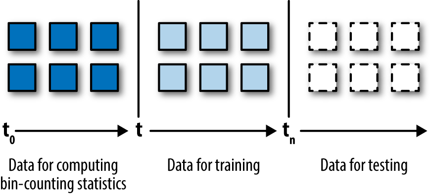
If the bin-counting procedure used the current data point’s label to compute part of the input statistic, that would constitute direct leakage. One way to prevent that is by instituting strict separation between count collection (for computing bin-count statistics) and training, as illustrated in Figure 5-5—i.e., use an earlier batch of data points for counting, use the current data points for training (mapping categorical variables to historical statistics we just collected), and use future data points for testing. This fixes the problem of leakage, but introduces the aforementioned delay (the input statistics and therefore the model will trail behind current data).如果分箱计算使用当前数据点的标签来计算输入统计数据的一部分,那么这将构成直接的泄漏。防止这种情况的一种方法是在计数收集(为计算分箱计算统计量)和训练之间建立严格的分离,如图5-5所示,使用早期的一批数据点进行计数,使用当前的数据点进行训练(将分类变量映射到刚得到的统计量),并使用未来的数据点进行测试。
It turns out that there is another solution, based on differential privacy. A statistic is approximately leakage-proof if its distribution stays roughly the same with or without any one data point. In practice, adding a small random noise with distribution Laplace(0,1) is sufficient to cover up any potential leakage from a single data point. This idea can be combined with leaving-one-out counting to formulate statistics on current data (Zhang, 2015).还有其他方法,基于 。如果一个统计数据的分布在任何一个数据点下(或者去掉任何数据点)的分布保持大致相同,那么该统计数据就可以基本防止泄漏。在实践中,添加一个带有拉普拉斯(0,1)分布的小随机噪声就足以掩盖单个数据点的任何潜在泄漏。这一思想可以与“留一”计数相结合,形成关于当前数据的统计。(Zhang, 2015)
Counts without bounds计数没有界限
If the statistics are updated continuously given more and more historical data, the raw counts will grow without bounds. This could be a problem for the model. A trained model “knows” the input data up to the observed scale. A trained decision tree might say, “When x is greater than 3, predict 1.” A trained linear model might say, “Multiply x by 0.7 and see if the result is greater than the global average.” These might be the correct decisions when x lies between 0 and 5. But what happens beyond that? No one knows.如果统计数据不断更新,得到计数越来越多的历史数据,那么原始数据的数量将会无限增长。这对模型是个挑战。训练后的模型“知道”已见过数据的规模的输入数据。训练后的决策树模型可能会说:“当x大于3,预测1。”训练后的线性模型可能会说:“0.7乘以x,看结果是否大于全局平均数。”当x处在0到5之间时结果是对的。但超过范围会怎么样,没人知道。
When the input counts increase, the model will need to be retrained to adapt to the current scale. If the counts accumulate rather slowly, then the effective scale won’t change too fast, and the model will not need to be retrained too frequently. But when counts increment very quickly, frequent retraining will be a nuisance.当输入数据的计数增长,需要重新训练模型以适应现在的规模。如果计数累积很缓慢,那么系数的规模不会快速变化,不必频繁更新模型。但当计数迅速增加时,频繁的重训练将是一个麻烦。
For this reason, it is often better to use normalized counts that are guaranteed to be bounded in a known interval. For instance, the estimated click-through probability is bounded between [0, 1]. Another method is to take the log transform, which imposes a strict bound, but the rate of increase will be very slow when the count is very large.因此,通常最好使用保证在已知间隔内有界的规范化计数。例如,估计的点击通过概率在[0,1]之间。另一种方法是进行log变换,它有一个严格的界限,但是当计数非常大时,增长率会非常缓慢。
Neither method will guard against shifting input distributions (e.g., last year’s Barbie dolls are now out of style and people will no longer click on those ads). The model will need to be retrained to accommodate these more fundamental changes in input data distribution, or the whole pipeline will need to move to an online learning setting where the model is continuously adapting to the input.这两种方法都不能防止输入分布的变化(例如,去年的芭比娃娃已经过时了,人们将不再点击这些广告)。需要重新训练模型,以适应输入数据分布中的这些更基本的变化,否则整个管道将需要转移到在线学习环境,其中模型将不断地适应输入。
5.3 Summary总结
| Plain one-hot encoding原始独热编码 | |
|---|---|
| Space requirement | O(n) using the sparse vector format, where n is the number of data points |
| Computation requirement | O(nk) under a linear model, where k is the number of categories |
| Pros | 1.Easiest to implement实现最简单 2.Potentially most accurate可能最精确 3.Feasible for online learning网上学习可行 |
| Cons | 1.Computationally inefficient计算效率低下 2.Does not adapt to growing categories对分类增长不适应 3.Not feasible for anything other than linear models除了线性模型外,其它都不可行 4.Requires large-scale distributed optimization with truly large datasets需要具有真正大型数据集的大规模分布式优化 |
| Feature hashing特征哈希 | |
|---|---|
| Space requirement | O(n) using the sparse matrix format, where n is the number of data points |
| Computation requirement | O(nm) under a linear or kernel model, where m is the number of hash bins |
| Pros | 1.Easy to implement实现简单 2.Makes model training cheaper训练负担较小 3.Easily adaptable to new categories适应新的分类 4.Easily handles rare categories容易处理罕见分类 5.Feasible for online learning网上学习可行 |
| Cons | 1.Only suitable for linear or kernelized models只适应线性模型和核化的模型 2.Hashed features not interpretable哈希后的特征不易解释 3.Mixed reports of accuracy精度有一定差异 |
| Bin-counting分箱计算 | |
|---|---|
| Space requirement | O(n+k) for small, dense representation of each data point, plus the count statistics that must be kept for each category |
| Computation requirement | O(n) for linear models; also usable for nonlinear models such as trees |
| Pros | 1.Smallest computational burden at training time最小的计算负担和训练时间 2.Enables tree-based models可用于基于树的模型 3.Relatively easy to adapt to new categories相对容易适应新分类 4.Handles rare categories with back-off or count-min sketch可采用back-off或count-min sketch处理罕见分类 5.Interpretable可解释 |
| Cons | 1.Requires historical data要求历史数据 2.Delayed updates required, not completely suitable for online learning需要延迟更新,不完全适合在线学习 3.Higher potential for leakage很可能泄露 |
5.4 Bibliography文献目录
6 Dimensionality Reduction: Squashing the Data Pancake with PCA降维:用PCA压碎数据煎饼
frequency-based filtering might say, “Get rid of all counts that are smaller than n,” a procedure that can be carried out without further input from the data itself.基于频率的过滤可能会说,去掉所有小于n的计数,这个过程无需数据本身的进一步输入即可执行。
Model-based techniques, on the other hand, require information from the data. For example, PCA is defined around the principal axes of the data. 另一方面,基于模型的技术需要来自数据的(全部)信息。例如,PCA是围绕数据的主轴定义的。
6.1 Intuition直觉
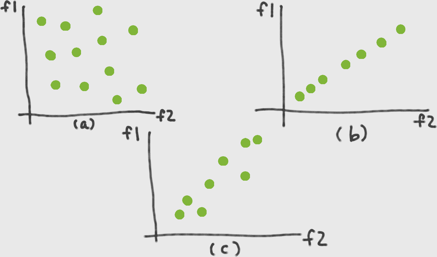
Dimensionality reduction is about getting rid of “uninformative information” while retaining the crucial bits. There are many ways to define “uninformative.” PCA focuses on the notion of linear dependency. If the column space is small compared to the total number of features, then most of the features are linear combinations of a few key features. Linearly dependent features are a waste of space and computation power because the information could have been encoded in much fewer features. To avoid this situation, principal component analysis tries to reduce such “fluff” by squashing the data into a much lower-dimensional linear subspace.降维是在保留关键位的同时去掉不提供信息的信息。有很多方法可以定义“无信息”。PCA侧重于线性依赖的概念。如果列空间与特征的总数相比很小,那么大多数特征是一些关键特征的线性组合。线性相关的特征是对空间和计算能力的浪费,因为信息可以编码在更少的特征中。为了避免这种情况,主成分分析试图通过将数据压缩到一个更低维的线性子空间来减少这种混乱。
6.2 Derivation推导
let X denote the n × d data matrix, where n is the number of data points and d the number of features. Let x be a column vector containing a single data point. (So x is the transpose of one of the rows in X.) Let v denote one of the new feature vectors, or principal components, that we are trying to find.设X为n乘以d数据矩阵,其中n为数据点数,d为特征数。设x为包含单个数据点的列向量(这样x是X其中一行的转置)。v表示我们要找的一个新的特征向量,或主成分。
Singular Value Decomposition (SVD) of a Matrix矩阵奇异值分解(SVD)
Any rectangular matrix can be decomposed into three matrices of particular shapes and characteristics: $$X = U Σ V^T$$ Here, U and V are orthogonal matrices (i.e., $$U^T U = I$$ and $$V^T V = I$$). Σ is a diagonal matrix containing the singular values of X, which can be positive, zero, or negative. Suppose X has n rows and d columns and n ≥ d. Then U has shape n × d, and Σ and V have shape d × d. (See “Singular Value Decomposition (SVD)” for a full review of SVD and eigen decomposition of a matrix.)
任何矩形矩阵都可以分解为三个具有特定形状和特征的矩阵: $$X = U Σ V^T$$ 这里U和V是正交矩阵($$U^T U = I$$,$$V^T V = I$$)。Σ是一个对角矩阵,其中包含X的奇异值,它可以是正、零、负。假设X有n行d列且n ≥ d。U形状为n乘以d,Σ、V形状为d乘以d。(参阅“Singular Value Decomposition (SVD)”以获得对矩阵SVD和特征分解很高的完整了解。)
6.2.1 Linear Projection线性投影
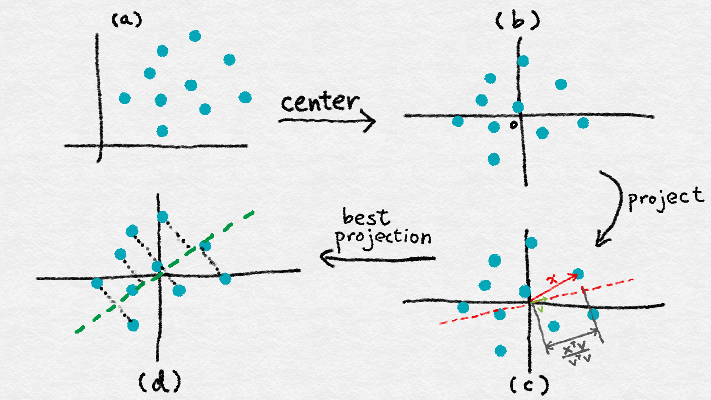
PCA uses linear projection to transform data into the new feature space. Figure 6-2(c) illustrates what a linear projection looks like. When we project x onto v, the length of the projection is proportional to the inner product between the two, normalized by the norm of v (its inner product with itself). Later on, we will constrain v to have unit norm. So, the only relevant part is the numerator—let’s call it v (see Equation 6-1).PCA利用线性投影将数据转换为新的特征空间。图6-2(c)展示了线性投影的样子。当我们把x投影到v上时,投影的长度与两者之间的内积成正比,由v的范数标准化(v的范数也就是v与自己的内积)。稍后,我们将约束v为单位范数。唯一相关的部分是分子我们叫它v(参考公式6-1)。
Equation 6-1. Projection coordinate投影坐标 $$z = x^T v$
Note that z is a scalar, whereas x and v are column vectors. Since there are a bunch of data points, we can formulate the vector z of all of their projection coordinates on the new feature v (Equation 6-2). Here, X is the familiar data matrix where each row is a data point. The resulting z is a column vector.注意z是标量,而x和v是列向量。因为有很多数据点,我们可以在新特征v上表示出所有投影坐标的向量z(等式6-2)。这里,X是熟悉的数据矩阵,其中每一行都是一个数据点。得到的z是一个列向量。
Equation 6-2. Vector of projection coordinates向量的投影坐标 $$z = X v$$
6.2.1 Variance and Empirical Variance方差和经验方差
The next step is to compute the variance of the projections. Variance is defined as the expectation of the squared distance to the mean (Equation 6-3).下一步是计算投影的方差。这里方差定义为到均值的平方距离的期望。(等式6-3)
Equation 6-3. Variance of a random variable Z随机变量Z的方差 Var(Z) = E[Z – E(Z)]2
There is one tiny problem: our formulation of the problem says nothing about the mean, E(Z); it is a free variable. One solution is to remove it from the equation by subtracting the mean from every data point. The resulting dataset has mean zero, which means that the variance is simply the expectation of Z2. Geometrically, subtracting the mean has the effect of centering the data. (See Figure 6-2(a-b).)有个小问题:我们对问题的表述没有提到均值E(Z),它是一个自由变量。一种解决方法是通过从每个数据点减去平均值,将其从方程中去掉。结果数据集的平均值为零,这意味着方差仅仅是Z2的期望。从几何上讲,减去均值具有数据中心的作用。
A closely related quantity is the covariance between two random variables Z1 and Z2 (Equation 6-4). Think of this as the extension of the idea of variance (of a single random variable) to two random variables.一个密切相关的量是两个随机变量Z1和Z2之间的协方差(等式6-4)。把这个看成是方差(单个随机变量)的概念扩展到两个随机变量。
Equation 6-4. Covariance between two random variables Z1 and Z2两个随机变量Z1和Z2的协方差 Cov(Z1, Z2) = E[(Z1 – E(Z1)(Z2 – E(Z2)] When the random variables have mean zero, their covariance coincides with their linear correlation, E[Z1Z2]. We will discuss this concept more later on.当随机变量的均值为零时,其协方差与线性相关即E[Z1Z2]一致。稍后我们将进一步讨论这个概念。
Statistical quantities like variance and expectation are defined on a data distribution. In practice, we don’t have the true distribution, but only a bunch of observed data points, z1, ..., zn. This is called an empirical distribution, and it gives us an empirical estimate of the variance (Equation 6-5).方差和期望等统计量是对数据分布定义的。在实践中,我们没有真正的分布,但是只有一些观察到的数据点,$z_1$到$z_n$。这被称为经验分布,它给出了方差的经验估计(方程6-5)。
Equation 6-5. Empirical variance of Z based on observations z基于观测值z的Z的经验方差 $$Var emp (Z) = 1/(n–1) ∑ i=1 ^n z_i^2$$
6.2.1 Principal Components: First Formulation主成分:第一方程式
Combined with the definition of $z_i$ in Equation 6-1, we have the formulation for maximizing the variance of the projected data given in Equation 6-6. (We drop the denominator n–1 from the definition of empirical variance, because it is a global constant and does not affect where the maximizing value occurs.)结合式(6-1)中$z_i$的定义,我们得到了使公式(6-6)中投影数据方差最大化的公式。(我们将分母n-1从经验方差的定义中去掉,因为它是一个全局常数,不影响最大值发生的位置。)
Equation 6-6. Objective function of principal components主成分的目标函数(寻找w,使w与$x_i$的内积的平方和最大,其中w的范数为1) $$max_w ∑ _ i=1 ^n ( x _ i^T w ) ^2 , where w^T w=1$$
The constraint here forces the inner product of w with itself to be 1, which is equivalent to saying that the vector must have unit length. This is because we only care about the direction and not the magnitude of w. The magnitude of w is an unnecessary degree of freedom, so we get rid of it by setting it to an arbitrary value.这里的约束条件迫使w与自身的内积为1,这等价于向量必须有单位长度。这是因为我们只关心方向而不关心w的大小。w的大小是一个不必要的自由度,所以我们把它设为武断值1就可以去掉。
6.2.1 Principal Components: Matrix-Vector Formulation主成分:矩阵-向量方程式
Next comes the tricky step. The sum of squares term in Equation 6-6 is rather cumbersome. It’d be much cleaner in a matrix-vector format.The key lies in the sum-of-squares identity: the sum of a bunch of squared terms is equal to the squared norm of a vector whose elements are those terms, which is equivalent to the vector’s inner product with itself. With this identity in hand, we can rewrite Equation 6-6 in matrix-vector notation, as shown in Equation 6-7.接下来是棘手的一步。方程6-6的平方和相当繁琐。它在矩阵-向量格式中更简洁。关键在于平方和恒等式:一堆项目的平方和等于这些项目组成的向量的平方范数,向量的平方范数也就是向量与其本身的内积。
关键在于平方和恒等式:一堆平方项的和等于一个元素是这些项的向量的平方范数,它等于向量s与自身的内积。
Equation 6-7. Objective function for principal components, matrix-vector formulation主成分的目标函数,矩阵-向量形式(寻找w,使最大,其中)这两个公式有问题,但话说回来向量的优化怎么求? $$max_w w^T w, where w^T w = 1$$ This formulation of PCA presents the target more clearly: we look for an input direction that maximizes the norm of the output. Does this sound familiar? The answer lies in the singular value decomposition (SVD) of X. The optimal w, as it turns out, is the principal left singular vector of X, which is also the principal eigenvector of $X^T X$. The projected data is called a principal component of the original data.这个关于PCA的方程式将目标清晰呈现:寻找输入方向以最大化输出的范数。听起来很熟悉吧?答案就是X的奇异值分解(SVD)。最优w是X的主左奇异向量,也是$X^T X$的主特征向量。投影数据称为原始数据的主成分。
6.2.1 General Solution of the Principal Components主成分的总体解决方案
This process can be repeated. Once we find the first principal component, we can rerun Equation 6-7 with the added constraint that the new vector be orthogonal to the previously found vectors (see Equation 6-8).这个过程可以重复。一旦我们找到了第一个主分量,我们就可以重新运行方程6-7,加上一个约束条件,即新向量与先前发现的向量正交(见方程6-8)。
Equation 6-8. Objective function for k+1st principal components第k+1个主成分的目标函数(寻找w,使最大,其中)这两个公式有问题,但话说回来向量的优化怎么求? $$max_w w_T w, where wTw = 1 and w^T w_1 = ... = w^T w_k = 0$$ The solution is the k+1st left singular vectors of X, ordered by descending singular values. Thus, the first k principal components correspond to the first k left singular vectors of X.解出的是按奇异值降序排列的,X的第k+1个左奇异向量。因此,前一个k个主分量对应于X的前k个左奇异向量。
6.2.1 Transforming Features转换特征
Once the principal components are found, we can transform the features using linear projection. Let $X = U Σ V^T$ be the SVD of X, and Vk the matrix whose columns contain the first k left singular vectors. X has shapes n × d, where d is the number of original features, and Vk has shapes d × k. Instead of a single projection vector as in Equation 6-2, we can simultaneously project onto multiple vectors in a projection matrix (Equation 6-9).一旦找到主分量,我们就可以用线性投影变换特征。让$X = U Σ V^T$是X的奇异值分解,$V_k$矩阵的列包括前k个左奇异向量。X的形状为n乘以d,其中d为原始特征数目,$V_k$的形状为d乘以k。与方程6-2中的单个投影向量不同,我们可以同时投影到投影矩阵中的多个向量(方程6-9)。
Equation 6-9. PCA projection matrix PCA投影矩阵 $$W = V_k$$ The matrix of projected coordinates is easy to compute, and can be further simplified using the fact that the singular vectors are orthogonal to each other (see Equation 6-10).投影坐标系的矩阵很容易计算,并且可以利用奇异向量彼此正交的事实进一步简化(方程6-10)。 Equation 6-10. Simple PCA transform简单PCA转换 $$Z = XW = X V_k = U Σ V^T V_k = U_k Σ_k$$ The projected values are simply the first k right singular vectors scaled by the first k singular values. Thus, the entire PCA solution, components and projections alike, can be conveniently obtained through the SVD of X.投影的值就是前k个右奇异向量乘以前k个奇异值。因此,通过SVD可以方便地获X的得整个PCA解决方案、成分和投影。
6.2.1 Implementing PCA应用主成分分析PCA
Many derivations of PCA involve first centering the data, then taking the eigen decomposition of the covariance matrix. But the easiest way to implement PCA is by taking the singular value decomposition of the centered data matrix.PCA的很多推导都是先中心化数据,然后对协方差矩阵进行特征分解。但实现PCA最简单的方法是对中心化后的数据矩阵进行奇异值分解。
PCA Implementation Steps 1. Center the data matrix:中心化数据矩阵: $$C = X – 1 μ^T$$ where 1 is a column vector containing all 1s, and μ is a column vector containing the average of the rows of X.其中1是全含1的列向量,μ是含有X行均值的列向量。 2. Compute the SVD:计算SVD: $$C = U Σ V^T$$ 3. Find the principal components. The first k principal components are the first k columns of V; i.e., the right singular vectors corresponding to the k largest singular values.寻找主成分。前k个主成分即V的前k列;例如,右奇异向量对应最大k个奇异值。 4. Transform the data. The transformed data is simply the first k columns of U. (If whitening is desired, then scale the vectors by the inverse singular values. This requires that the selected singular values are nonzero. See “Whitening and ZCA”.)转换数据。转换后的数据即U的前k列。(如果需要白化,则用逆奇异值对向量进行缩放。这要求所选奇异值是非零的。请阅读“Whitening and ZCA”)
6.3 PCA in Action主成分分析PCA实操
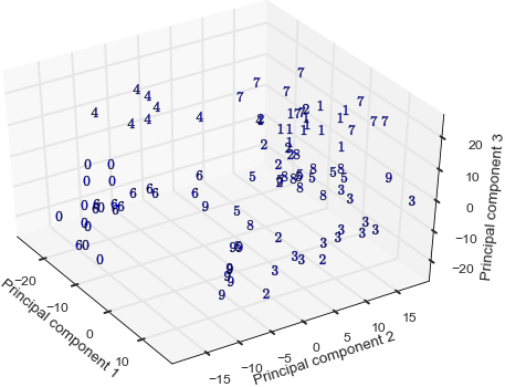
如图,PCA后可用较少维度呈现数据,又不丢失很多信息。
6.4 Whitening and ZCA白化和ZCA
Due to the orthogonality constraint in the objective function, PCA transformation produces a nice side effect: the transformed features are no longer correlated. In other words, the inner products between pairs of feature vectors are zero. It’s easy to prove this using the orthogonality property of the singular vectors:由于目标函数的正交性约束,PCA变换产生了很好的副作用:变换后的特征不再相关。换句话说,特征向量对之间的内积为零。利用奇异向量的正交性性质很容易证明这一点:
$$ZTZ = Σ_k U_k^T U_k Σ_k = Σ_k^2$$ The result is a diagonal matrix containing squares of the singular values representing the correlation of each feature vector with itself, also known as its ℓ2 norm.结果是一个对角矩阵,其中包含表示每个特征向量对应的奇异值的平方,也称为其ℓ2范数。
Sometimes, it is useful to also normalize the scale of the features to 1. In signal processing terms, this is known as whitening. It results in a set of features that have unit correlation with themselves and zero correlation with each other. Mathematically, whitening can done by multiplying the PCA transformation with the inverse singular values (see Equation 6-11).有时,还可以将特征的规模规范化为1。在信号处理术语中,这被称为白化。这导致特征与本身具有单位相关性,彼此之间的相关性为零。从数学上讲,白化可以通过将PCA变换与逆奇异值相乘来实现(方程6-11)。
Equation 6-11. PCA + whitening $$W_white = V_k Σ_k^-1$$ $$Z_white = X V_k Σ_k^-1 = U Σ V^T V_k Σ_k^-1 = U_k$$ Whitening is independent from dimensionality reduction; one can perform one without the other. For example, zero-phase component analysis (ZCA) (Bell and Sejnowski, 1996) is a whitening transformation that is closely related to PCA, but that does not reduce the number of features. ZCA whitening uses the full set of principal components V without reduction, and includes an extra multiplication back onto $V^T$ (Equation 6-12).白化与降维无关,两者可只进行一种。例如,零相位成分分析(ZCA)(Bell和Sejnowski, 1996)是一种接近PCA的白化转换,但ZCA不减少特征。ZCA白化使用全部主成分V而不删减主成分,并且包括一个额外的乘项$V^T$(方程6-12)。 Equation 6-12. ZCA whitening $$W_ZCA = V Σ^-1 V^T$$ $$Z_zca = X V Σ^-1 V^T = U Σ V^T V Σ^-1 V^T = U V^T$$
Simple PCA projection (Equation 6-10) produces coordinates in the new feature space, where the principal components serve as the basis. These coordinates represent only the length of the projected vector, not the direction. Multiplication with the principal components gives us the length and the orientation. Another valid interpretation is that the extra multiplication rotates the coordinates back into the original feature space. (V is an orthogonal matrix, and orthogonal matrices rotate their input without stretching or compression.) So, ZCA produces whitened data that is as close (in Euclidean distance) to the original data as possible.简单的PCA投影(方程6-10)在新特征空间中产生坐标,主成分作为基础。这些坐标只代表投影向量的长度,而不是方向。与主成分相乘得到长度和方向。另一个有效的解释是,额外的乘法将坐标旋转回原始特征空间(V是一个正交矩阵,正交矩阵在不拉伸或压缩的情况下旋转它们的输入。)。因此,ZCA生成尽可能接近(欧几里德距离)原始数据的白色数据。
6.5 Considerations and Limitations of PCA主成分分析PCA的注意事项和限制
One key criticism of PCA is that the transformation is fairly complex, and the results are therefore hard to interpret. The principal components and the projected vectors are real-valued and could be positive or negative. The principal components are essentially linear combinations of the (centered) rows, and the projection values are linear combinations of the columns.对PCA的一个关键批评是,转换相当复杂,因此结果很难解释。主成分和投影向量都是实值的,可以是正的,也可以是负的。主分量本质上是(中心化了的)行的线性组合,投影值是列的线性组合。
PCA is computationally expensive. It relies on SVD, which is an expensive procedure. To compute the full SVD of a matrix takes $O(n d^2 + d^3)$ operations (Golub and Van Loan, 2012), assuming n ≥ d—i.e., there are more data points than features. Even if we only want k principal components, computing the truncated SVD (the k largest singular values and vectors) still takes O((n+d)2 k) = O(n2k) operations. This is prohibitive when there are a large number of data points or features.PCA在计算上非常昂贵。它依赖于SVD,这是一个昂贵的过程。完全计算矩阵的SVD需$O(n d^2 + d^3)$步操作(Golub和Van Loan, 2012),假设n ≥ d,那么数据点数大于特征数。即使我们只需要k个主成分,计算截断SVD(前k个最大奇异值和奇异向量)仍需$O((n+d)^2 k) = O(n^2 k)$步操作。当有大量的数据点或特性时,这是禁止的。
Lastly, it is best not to apply PCA to raw counts (word counts, music play counts, movie viewing counts, etc.). The reason for this is that such counts often contain large outliers. As we know, PCA looks for linear correlations within the features. Correlation and variance statistics are very sensitive to large outliers; a single large number could change the statistics a lot. So, it is a good idea to first trim the data of large values (“Frequency-Based Filtering”), or apply a scaling transform like tf-idf (Chapter 4) or the log transform (“Log Transformation”).最后,最好不要对原始计数(如字数计数、音乐点击计数、电影观看量计数等)进行PCA。原因是这类计数通常含有大量域外值,一个很大的值就能明显改变统计量。因此,最好先对大值数据进行修剪(“Frequency-Based Filtering”)或先进行如tf-idf(第四章)缩放转换,或对数转换(“Log Transformation”)。
6.6 Use Cases使用案例
PCA transformation discards information from the data. Thus, the downstream model may be cheaper to train, but less accurate. PCA转换丢弃数据中的信息。因此,训练得到的的训练成本可能更低,但准确率较低。
One of the coolest applications of PCA is in anomaly detection of time series.PCA最有趣的应用之一是时间序列的异常检测。
PCA is also often used in financial modeling. In those use cases, it works as a type of factor analysis, a term that describes a family of statistical methods that aim to describe observed variability in data using a small number of unobserved factors. In factor analysis applications, the goal is to find the explanatory components, not the transformed data.PCA也经常用于金融建模。在这些用例中,它作为一种因子分析,这个术语描述了一系列统计方法,目的是使用少量未观察到的因素来描述数据中观察到的可变性。在因子分析应用程序中,目标是找到解释成分,而不是得到转换后的数据。
Financial quantities like stock returns are often correlated with each other. Stocks may move up and down at the same time (positive correlation), or move in opposite directions (negative correlation). In order to balance volatility and reduce risk, an investment portfolio needs a diverse set of stocks that are not correlated with each other. (Don’t put all your eggs in one basket if that basket is going to sink.) Finding strong correlation patterns is helpful for deciding on an investment strategy.像股票收益这样的金融数据通常是相互关联的。股票可以同时上下波动(正相关),也可以反向波动(负相关)。为了平衡波动和降低风险,一个投资组合需要一组不同的股票,它们彼此之间不相关(不要把所有的鸡蛋放在一个篮子里,如果篮子要沉的话。)。发现强相关性模式有助于决定投资策略。
Stock correlation patterns can be industry-wide. For example, tech stocks may go up and down together, while airline stocks tend to go down when oil prices are high. But industry may not be the best way to explain the outcome. Analysts also look for unexpected correlations in observed statistics. In particular, the statistical factor model (Connor, 1995) runs PCA on the matrix of time series of individual stock returns to find commonly covarying stocks. In this use case, the end goal is the principal components themselves, not the transformed data.股票相关模式可以是全行业的。例如,科技股可能同时涨跌,而航空股在油价高企时往往会下跌。但行业可能不是解释结果的最佳方式。分析师还会在观察到的统计数据中寻找出人意料的相关性。特别地,统计因子模型(Connor, 1995)在单个股票收益的时间序列矩阵上运行PCA来寻找一般共变股票。在这个用例中,最终目标是主成分本身,而不是转换后的数据。
ZCA is useful as a preprocessing step when learning from images. In natural images, adjacent pixels often have similar colors. ZCA whitening can remove this correlation, which allows subsequent modeling efforts to focus on more interesting image structures. 当从图像中学习时,ZCA是一个很有用的预处理步骤。在自然图像中,相邻像素通常具有相似的颜色。ZCA白化可以消除这种相关性,从而允许后续的建模工作将重点放在更有趣的图像结构上。
Many deep learning models use PCA or ZCA as a preprocessing step, though it is not always necessary. Whitening is not necessary but speeds up the convergence of the algorithm. 许多深度学习模型使用PCA或ZCA作为预处理步骤,尽管并不总是必要的。白化不是必须的,但加速了算法的收敛。
6.7 Summary总结
PCA is a well-known dimensionality reduction method. But it has its limitations, such as high computational cost and uninterpretable outcome. It is useful as a preprocessing step, especially when there are linear correlations between features.PCA是一种著名的降维方法。但它也有它的局限性,比如高计算成本和不可解释的结果。它作为预处理步骤非常有用,特别是当特征之间存在线性相关时。
Its cousin, ZCA, whitens the data in an interpretable way, but does not reduce dimensionality.与PCA类似的ZCA,以可解释的方式使数据白化,但不减少维数。
6.8 Bibliography文献目录
7 Nonlinear Featurization via K-Means Model Stacking 通过k-均值模型堆叠进行非线性特征化
PCA is very useful when the data lies in a linear subspace like a flat pancake. But what if the data forms a more complicated shape? A flat plane (linear subspace) can be generalized to a manifold (nonlinear subspace), which can be thought of as a surface that gets stretched and rolled in various ways.当数据像扁平煎饼一样位于线性子空间中时,PCA是非常有用的。但如果数据形成一个更复杂的形状呢?平面(线性子空间)可以推广到流形(非线性子空间),它可以被认为是一个以各种方式拉伸和滚动的曲面。
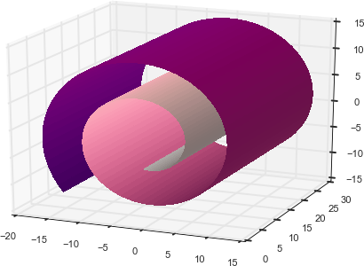 瑞士卷,非线性流形
Nonlinear dimensionality reduction is also called nonlinear embedding or manifold learning.非线性降维也称为非线性嵌入或流形学习。
The goal of feature engineering, however, isn’t so much to make the feature dimensions as low as possible, but to arrive at the right features for the task. the right features are those that represent the spatial characteristics of the data.然而,特性工程的目标并不是使特性维度尽可能低,而是为任务找到正确的特性。正确的特征是表示数据空间特点的特征。
Clustering algorithms are usually not presented as techniques for local structure learning. But they in fact enable just that. Points that are close to each other (where “closeness” can be defined by a chosen metric) belong to the same cluster. Given a clustering, a data point can be represented by its cluster membership vector. If the number of clusters is smaller than the original number of features, then the new representation will have fewer dimensions than the original; the original data is compressed into a lower dimension. 聚类算法通常不作为局部结构学习的技术。但事实上,他们恰恰做到了这一点。彼此接近(接近程度由选定的度量尺度定义)的数据点属于同一聚类。给定一个聚类,一个数据点可以用它的聚类隶属向量来表示。如果聚类的数量小于原始特征的数量,那么新表示的维数将小于原始特征的维数;原始数据被压缩到一个较低的维度。
7.1 k-Means Clustering k-均值聚类
A clustering algorithm depends on a metric—a measurement of closeness between data points. The most popular metric is the Euclidean distance or Euclidean metric. 聚类算法依赖度量尺度-测量数据点之间的紧密度。最流行的度量尺度是欧式距离或称欧式度量尺度。
k-means establishes a hard clustering, meaning that each data point is assigned to one and only one cluster. The algorithm learns to position the cluster centers such that the total sum of the Euclidean distance between each data point and its cluster center is minimized. k-means建立了一个硬集群,这意味着每个数据点被分配给一个且只有一个集群。该算法学习了对聚类中心的定位,以使所有数据点与其聚类中心之间的欧氏距离之和最小。
注意:按我理解,k-means甚至可以不使用欧式距离来度量,也可以采用其他距离来度量嘛;而且可采用欧式距离度量的也不止K-means,K-medoids也可以。 又有表示k-means必须使用欧式距离度量尺度。
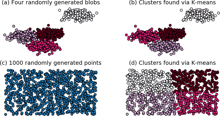 上图演示了聚类算法如何划分空间
7.2 Clustering as Surface Tiling聚类为表面平铺
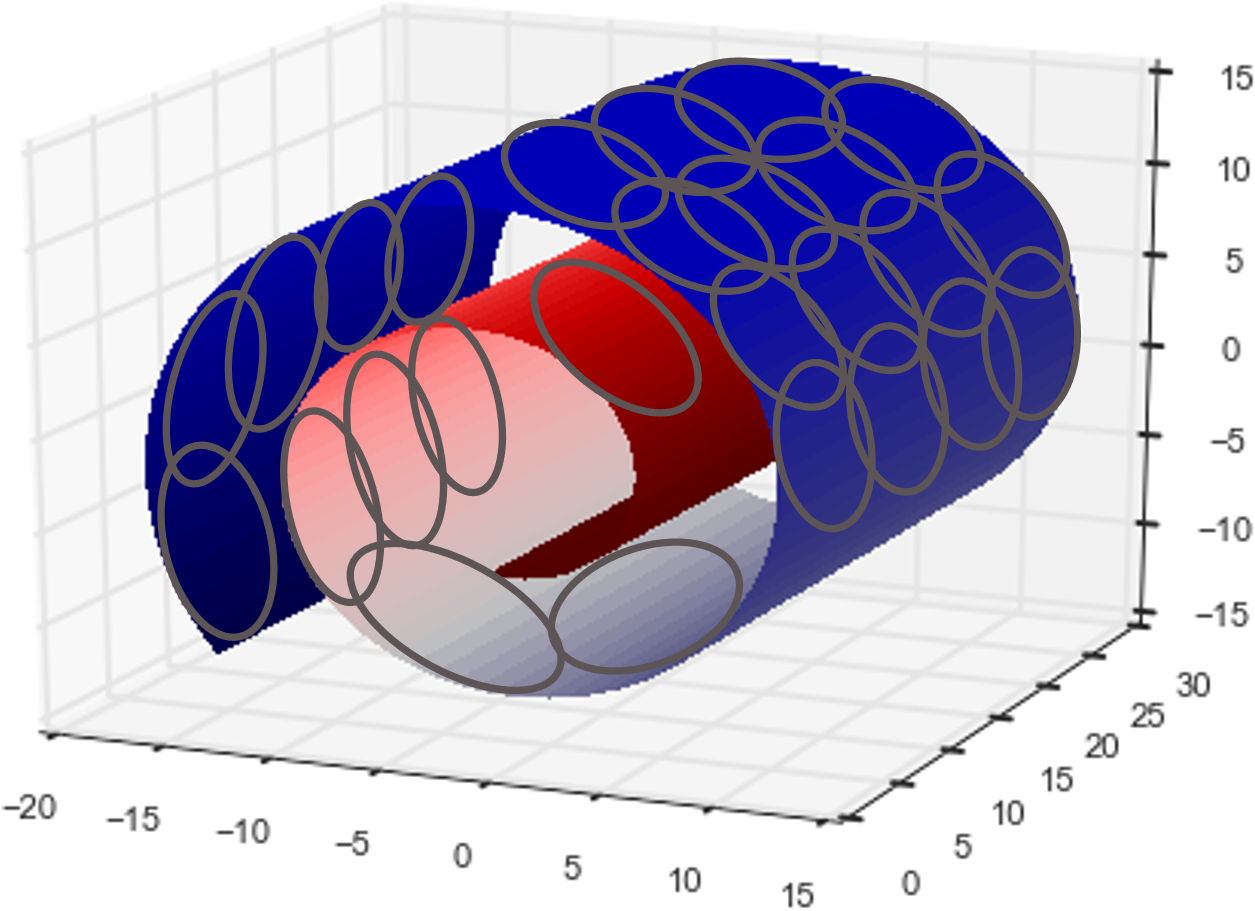
上图显示:聚类算法在概念上相当于给数据(如瑞士卷类的数据)分斑块
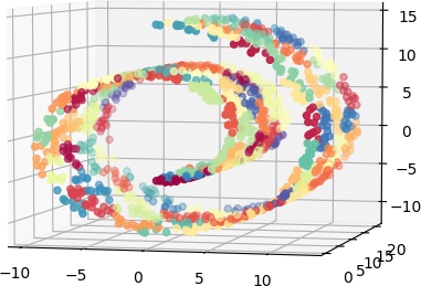
上图显示:100个聚类来近似表达瑞士卷数据集
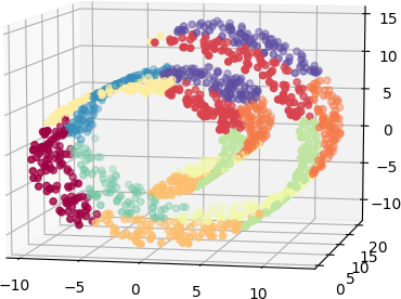
上图显示:10个聚类来近似表达瑞士卷数据集
So, if we are willing to tolerate a maximum approximation error of r per data point, then the number of clusters is $O(1/r^d)$, where d is the dimension of the original feature space of the data.因此,如要承受每个数据点的最大逼近误差为r,那么聚类数量是$O(1/r^d)$,这里d是原始数据的特征空间的维度。(显然,聚类数量越多精度越高。但抱持着降维的目的,我们需要聚类数量小于d,这要让我们承受一定的误差。)
7.3 k-Means Featurization for Classification k-均值聚类用于分类
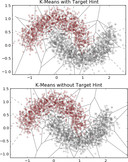
上图显示:有目标数据参与的分类比没有目标数据参与的分类更准确。
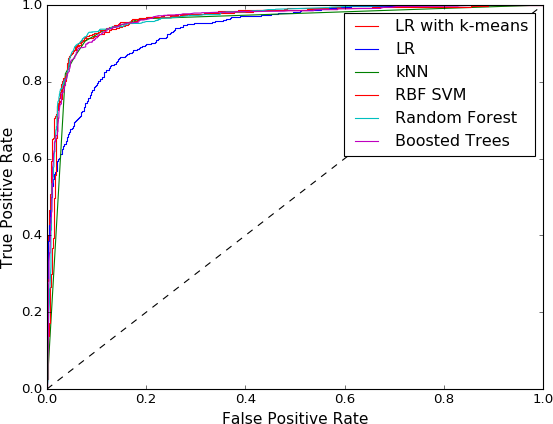
上图显示:LR+K-means(逻辑回归加有目标数据参与的k-Means特征化)的性能与非线性分类器(如KNN、RBF SVM、Random Forest、Boosted Trees等)相当,明显强于单纯LR(逻辑回归)。考虑到实际预测时候不可能给出目标数据target,即不可能有目标数据参与,我做实验发现其实没有目标数据参与的K-means特征化后LR结果与有目标参与是差不多的。
7.3.1 Alternative Dense Featurization 改用密集特征化
Instead of one-hot cluster membership, a data point can also be represented by a dense vector of its inverse distance to each cluster center. This retains more information than simple binary cluster assignment, but the representation is now dense. There is a trade-off here. One-hot cluster membership results in a very lightweight, sparse representation, but one might need a larger k to represent data of complex shapes. Inverse distance representation is dense, which could be more expensive for the modeling step, but one might be able to get away with a smaller k.除了使用独热聚类关系,还可以用到聚类中心距离的倒数来表示数据点。比简单的二进制集群分配保留了更多的信息,但现在这种表示是密集的了。这里有一个权衡。独热聚类成员关系会导致非常轻量级的稀疏表示,但是可能需要更大的k来表示复杂形状的数据。距离倒数表示是密集的,这可能对建模步骤更昂贵,但可以采用较小的k。
A compromise between sparse and dense is to retain inverse distances for only p of the closest clusters. But now p is an extra hyperparameter to tune. (Can you understand why feature engineering requires so much fiddling?) There is no free lunch. 稀疏和稠密之间的折衷办法是只保留p个最近簇的的距离倒数。但现在p是一个需要调整的高参。
7.4 Pros, Cons, and Gotchas正反方面和陷阱
Using k-means to turn spatial data into features is an example of model stacking, where the input to one model is the output of another. Another example of stacking is to use the output of a decision tree–type model (random forest or gradient boosting tree) as input to a linear classifier. Stacking has become an increasingly popular technique in recent years. Nonlinear classifiers are expensive to train and maintain. The key intuition with stacking is to push the nonlinearities into the features and use a very simple, usually linear model as the last layer. The featurizer can be trained offline, which means that one can use expensive models that require more computation power or memory but generate useful features. The simple model at the top level can be quickly adapted to the changing distributions of online data. This is a great trade-off between accuracy and speed, and this strategy is often used in applications like targeted advertising that require fast adaptation to changing data distributions.使用k-means将空间数据转换为特征是模型堆叠的一个例子,其中一个模型的输入是另一个模型的输出。另一个堆叠的例子是使用决策树类型模型(随机森林或梯度提升树)的输出作为线性分类器的输入。堆叠技术近年来已成为一种日益流行的技术。非线性分类器的训练和维护成本很高。堆叠的关键直觉是将非线性推入特征,并使用一个非常简单的,通常是线性模型作为最后一层。特征器可以离线训练,这意味着可以使用昂贵的模型,这些模型需要更多的计算能力或内存,但可以生成有用的特性。顶层的简单模型可以快速适应在线数据分布的变化。这是准确性和速度之间的巨大平衡,这种策略经常用于需要快速适应不断变化的数据分布的应用程序,比如目标广告。
| Model | Time | Space |
|---|---|---|
| k-means training | $O(n k d)$ | $O(k d)$ |
| k-means predict | $O(k d)$ | $O(k d)$ |
| LR + cluster features training | $O(n(d+k))$ | $O(d+k)$ |
| LR + cluster features predict | $O(d+k)$ | $O(d+k)$ |
| RBF SVM training | $O(n^2 d)$ | $O(n^2)$ |
| RBF SVM predict | $O(s d)$ | $O(s d)$ |
| GBT training | $O(n d 2^m t)$ | $O(nd + 2^m t)$ |
| GBT predict | $O(2^m t)$ | $O(2^m t)$ |
| kNN training | $O(1)$ | $O(n d)$ |
| kNN predict | $O(n d + k log n)$ | $O(n d)$ |
a Streaming k-means can be done in time O(n d (log k + log log n)), which is much faster than O(n k d) for large k.流动K-means计算更快。
Overall, k-means + LR is the only combination that is linear (with respect to the size of training data, O(nd), and model size, O(kd)) at both training and prediction time.总之,k-means + LR是在训练和预测时候都是线性的(相对训练数据和模型大小)。
Potential for Data Leakage数据泄漏的可能
Those who remember our caution regarding data leakage (see “Guarding against data leakage”) might ask whether including the target variable in the k-means featurization step would cause such a problem. The answer is “yes,” but not as much in the case of bin counting. If we use the same dataset for learning the clusters and building the classification model, then information about the target will have leaked into the input variables. As a result, accuracy evaluations on the training data will probably be overly optimistic, but the bias will go away when evaluating on a hold-out validation set or test set. Furthermore, the leakage will not be as bad as in the case of bin-counting statistics (see “Bin Counting”), because the lossy compression of the clustering algorithm will have abstracted away some of that information. To be extra careful about preventing leakage, hold out a separate dataset for deriving the clusters, just like in the case of bin counting.事实上K-means特征化时候引用目标变量将造成泄露,比分箱计算时轻微。如果我们使用相同的数据集来学习聚类和构建分类模型,那么关于目标的信息就会泄漏到输入变量中。因此,对训练数据的精确性评估可能会过于乐观,但是当在保留验证集或测试集上进行评估时,这种偏差将会消失。此外,泄漏不会像分箱计算统计信息那样严重(参见“Bin Counting”),因为聚类算法的有损压缩会抽象掉一些信息。为了防止泄漏,要格外小心,请拿出一个用于派生集群的单独数据集,就像二进制计数一样。
k-means featurization is useful for real-valued, bounded numeric features that form clumps of dense regions in space. The clumps can be of any shape, because we can just increase the number of clusters to approximate them. (Unlike in the classic clustering setup, we are not concerned with discovering the “true” number of clusters; we only need to cover them.)k-means特征化对于在空间中形成密集区域簇的实值有界数字特征非常有用。这些簇可以是任何形状,因为我们可以增加簇的数目来近似它们。(与经典的集群设置不同,我们不关心发现真正的集群数量;我们只需要覆盖它们。)
k-means cannot handle feature spaces where the Euclidean distance does not make sense—i.e., weirdly distributed numeric variables or categorical variables. If the feature set contains those variables, then there are several ways to handle them:k-means无法处理欧几里德距离没有意义的特征空间-例如,奇怪分布的数字变量或分类变量。如果特性集包含这些变量,那么有几种方法可以处理它们: * Apply k-means featurization only on the real-valued, bounded numeric features.仅在实值、有界数字特性上应用k-means特性化。 * Define a custom metric to handle multiple data types and use the k-medoids algorithms. (k-medoids is analogous to k-means but allows for arbitrary distance metrics.)定义一个定制的度量尺度来处理多个数据类型,并使用k-medoids算法。(k-medoids类似于k-means,但允许任意距离度量尺度。) * Convert categorical variables to binning statistics (see “Bin Counting”), then featurize them using k-means.将分类变量转换为分箱统计数据(参见“Bin Counting”),然后使用k-means对它们进行特性化。
Combined with techniques for handling categorical variables and time series, k-means featurization can be adapted to handle the kind of rich data that often appears in customer marketing and sales analytics. The resulting clusters can be thought of as user segments, which are very useful features for the next modeling step.结合处理分类变量和时间序列的技术,k-means特征化可以用来处理客户营销和销售分析中经常出现的丰富数据。
7.5 Summary总结
7.6 Bibliography文献目录
8 Automating the Featurizer: Image Feature Extraction and Deep Learning自动进行特征化:图像特征提取和深度学习
暂时不是我的兴趣点,有空再学

8.1 The Simplest Image Features (and Why They Don’t Work)最简单的图像特征(为什么不起作用?)
8.2 Manual Feature Extraction: SIFT and HOG人工特征提取:SIFT和HOG
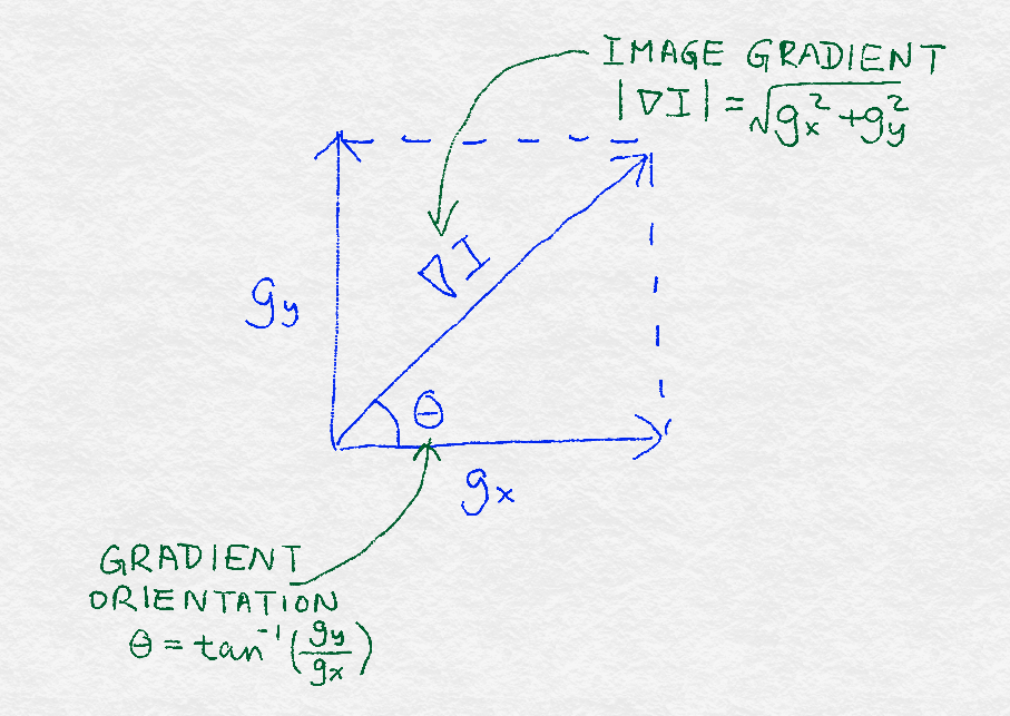
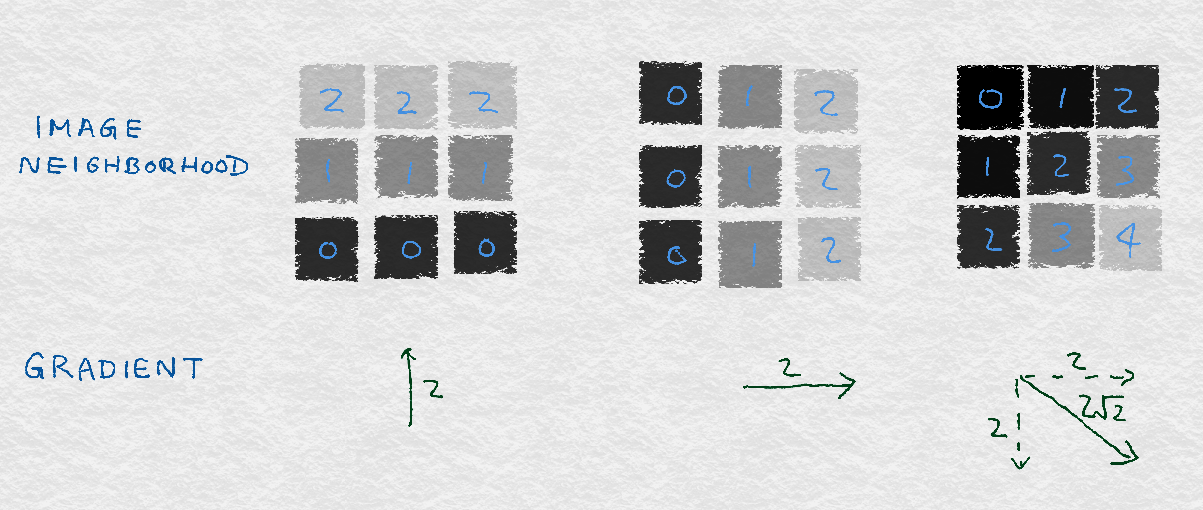
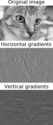
8.2.1 Image Gradients图像梯度
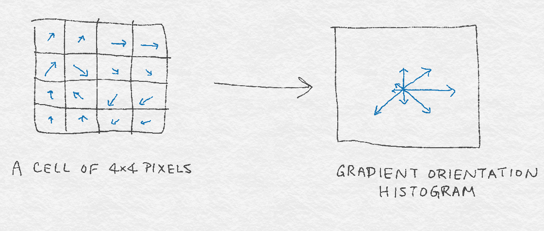
8.2.2 Gradient Orientation Histograms梯度方向直方图
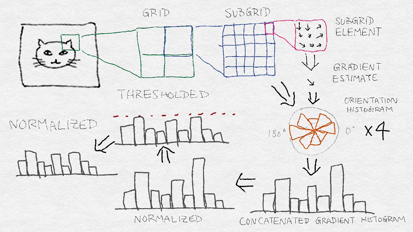
8.2.3 SIFT Architecture SIFT体系结构
8.3 Learning Image Features with Deep Neural Networks通过深度神经网络学习图像特征
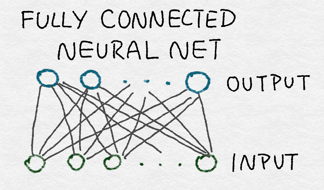
8.3.1 Fully Connected Layers全连接层
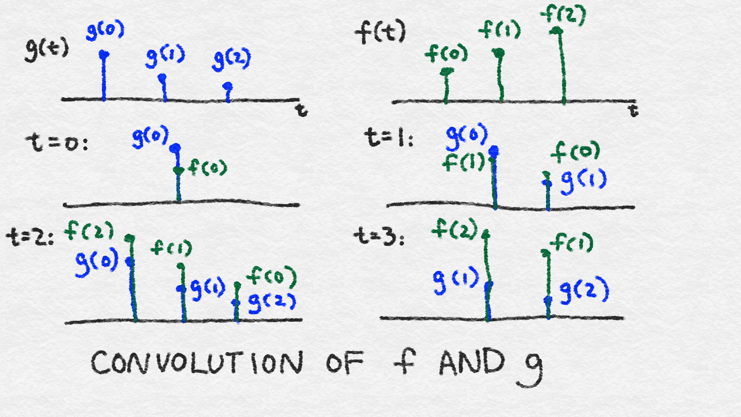
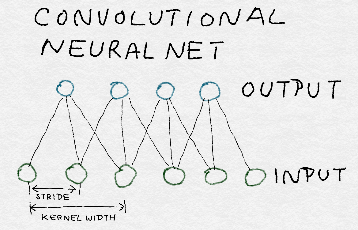
8.3.2 Convolutional Layers卷积层

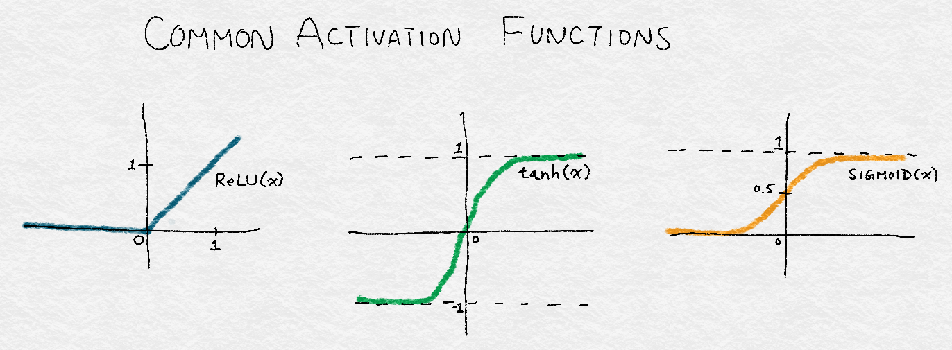
8.3.3 Rectified Linear Unit (ReLU) Transformation整流线性单元(ReLU)变换
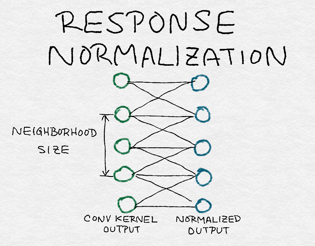
8.3.4 Response Normalization Layers应答规范化层
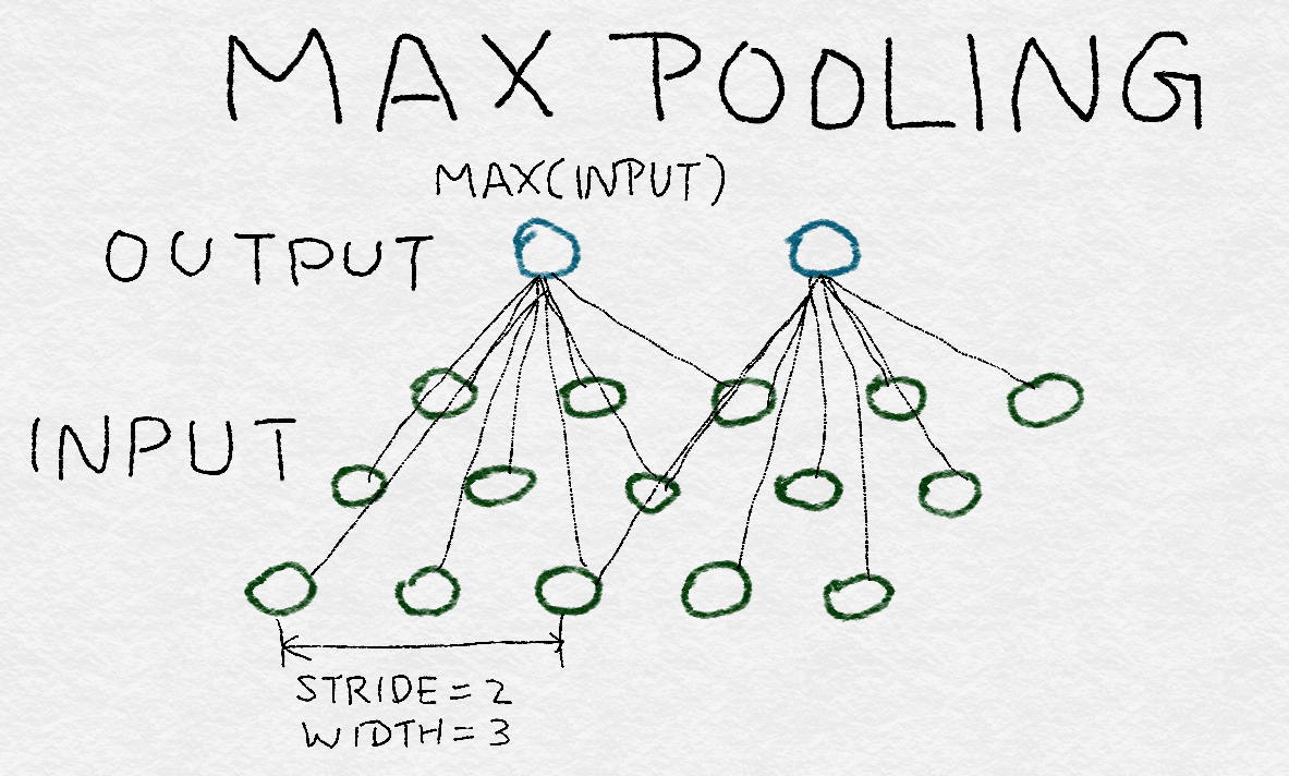
8.3.5 Pooling Layers池化层
8.3.6 Structure of AlexNet AlexNet结构
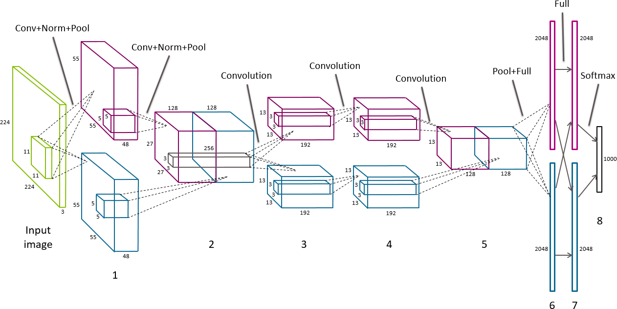
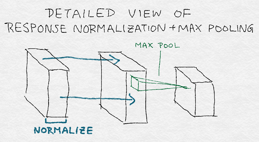
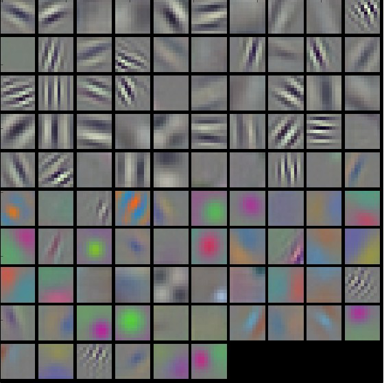

8.4 Summary总结
8.5 Bibliography文献目录
9 Back to the Feature: Building an Academic Paper Recommender回到特征:建立学术论文推荐系统
暂时不是我的兴趣点,有空再学
9.1 Item-Based Collaborative Filtering项目协同过滤
9.2 First Pass: Data Import, Cleaning, and Feature Parsing第一遍:对数据进行导入、清洗、特征解析
9.2.1 Academic Paper Recommender: Naive Approach学术论文推荐系统:朴素途径
9.3 Second Pass: More Engineering and a Smarter Model第二遍:更多引擎和一个更聪明的模型
9.3.1 Academic Paper Recommender: Take 2学术论文推荐系统:采用两个特征
9.4 Third Pass: More Features = More Information第二遍:更多特征=更多信息
9.4.1 Academic Paper Recommender: Take 3学术论文推荐系统:采用三个特征
9.5 Summary总结
9.6 Bibliography文献目录
Appendix A. Linear Modeling and Linear Algebra Basics线性建模和线性代数基础
A.1 Overview of Linear Classification线性分类概述
The points right on the cusp of being in one class versus another form a decision surface (Figure A-1).处于不同分类交界处的点形成一个决策面(图A-1)。
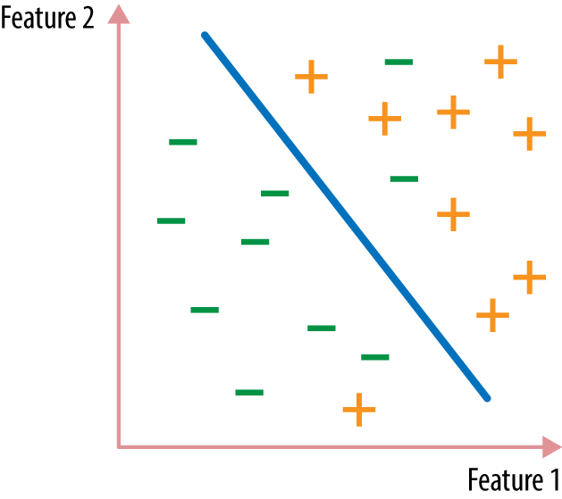
First of all, it’s easier to find the best simple separator than the best complex separator. Also, simple functions often generalize better to new data, because it’s harder to tailor them too specifically to the training data (a concept known as overfitting).首先,找到最好的简单分类器比找到最好的复杂分类器更容易。此外,简单函数通常更适应新数据,因为简单函数无法对训练数据特别定制(这是一个被称为过拟合的概念)。
The principle of minimizing complexity and maximizing usefulness is called “Occam’s razor,” and is widely applicable in science and engineering.最小化复杂性和最大化有用性的原则被称为奥卡姆剃刀,广泛应用于科学和工程领域。
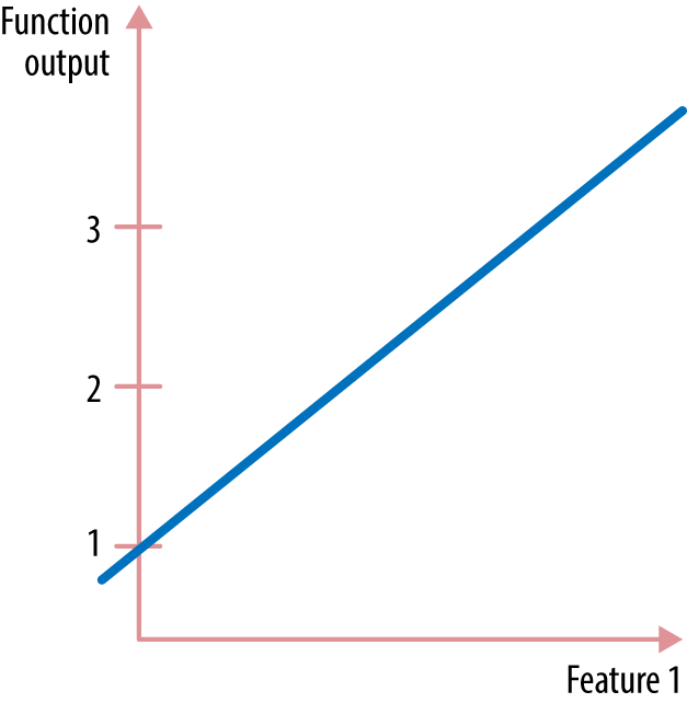
The simplest function is a line. A linear function of one input variable is a familiar sight (Figure A-2).最简单的函数是直线。一个输入变量的线性函数是一个熟悉的场景(图A-2)。
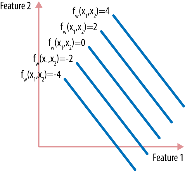
A linear function with two input variables can be visualized as either a flat plane in 3D or a contour plot in 2D (shown in Figure A-3).一个具有两个输入变量的线性函数可以被可视化为三维平面或二维等高线图(如图A-3所示)。
Training a linear classifier is equivalent to picking out the best separating hyperplane between the classes. This translates into finding the best vector w that is oriented exactly right in space. Since each data point has a target label y, we could find a w that tries to directly emulate the target label:训练一个线性分类器相当于在两个类之间挑选出最好的超平面。这就意味着找到在空间中方向完全正确的最佳向量w。由于每个数据点都有一个目标标签y,我们可以找到一个试图直接模拟目标标签的w: $$x^T w = y$$ Since there is usually more than one data point, we want a w that simultaneously makes all of the predictions close to the target labels:因为通常不止一个数据点,所以我们需要一个w,同时使所有预测都接近目标标签: $$A w = y$$ Here, A is known as the data matrix (also known as the design matrix in statistics). It contains the data in a particular form: each row is a data point and each column a feature. 在这里,A被称为数据矩阵(在统计学中也称为设计矩阵)。它以特定的形式包含数据:每一行是一个数据点,每一列是一个特性。
A.2 The Anatomy of a Matrix矩阵的解剖
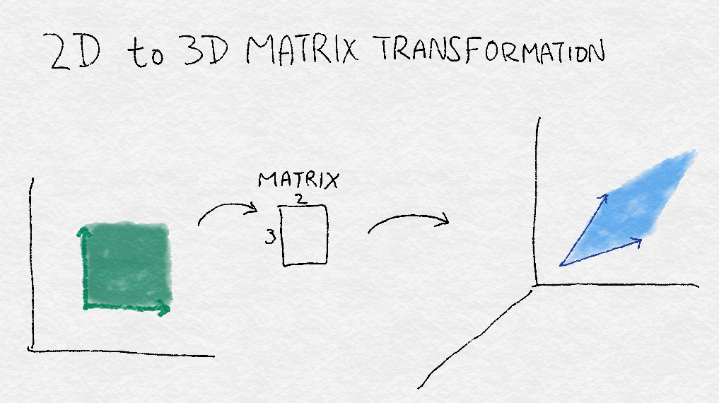
The equation states that when a certain matrix multiplies a certain vector, there is a certain outcome. A matrix is also called a linear operator, a name that makes it more apparent that a matrix is a little machine. This machine takes a vector as input and spits out another vector using a combination of several key operations: rotating a vector’s direction, adding or subtracting dimensions, and stretching or compressing its length.这个方程表明当一个矩阵乘以一个向量,就会得到一个结果。矩阵也被称为线性算子,这个名字使得矩阵更明显地是一个小机器。这台机器以一个向量作为输入,并使用几个关键操作组合出另一个向量:旋转一个向量的方向,增加或减少维度,拉伸或压缩它的长度。
For example, as Figure A-4 shows, a 3 × 2 matrix can transform a square area in 2D into a diamond-shaped area in 3D. It does so by rotating and stretching each vector in the input space into a new vector in the output space.例如,如图A-4所示,一个3乘以2矩阵可以将二维的正方形区域转换为三维的菱形区域。它通过将输入空间中的每个向量旋转并拉伸到输出空间中的一个新向量来实现。
A.2.1 From Vectors to Subspaces从向量到子空间
In order to understand a linear operator, we have to look at how it morphs the input into output. Luckily, we don’t have to analyze one input vector at a time. Vectors can be organized into subspaces, and linear operators manipulate vector subspaces.为了理解一个线性算子,我们必须看看它是如何把输入变成输出的。幸运的是,我们不必一次分析一个输入向量。向量可以被组织成子空间,线性算子处理向量子空间。
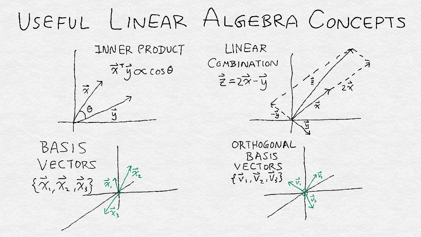
A subspace is a set of vectors that satisfies two criteria. First, if it contains a vector, then it contains the line that passes through the origin and that point. Second, if it contains two points, then it contains all the linear combinations of those two vectors. Linear combination is a combination of two types of operations: multiplying a vector with a scalar, and adding two vectors together.子空间是满足两个条件的向量的集合。首先,如果它包含一个向量,那么它包含经过原点和该向量代表的点的直线。第二,如果它包含两个点,那么它包含这两个向量的所有线性组合。线性组合是两种操作的组合:向量与标量相乘,以及两个向量相加。
One important property of a subspace is its rank or dimensionality, which is a measure of the degrees of freedom in this space. 子空间的一个重要性质是它的秩或维数,它是空间中自由度的度量。
“Independence” here means “linear independence”: two vectors are linearly independent if one isn’t a constant multiple of another (i.e., they are not pointing in exactly the same or opposite directions).独立在这里就是线性独立:两个向量线性独立,如果一个不是常数乘以另一个(例如他们方向不是完全相同或相反)。
A subspace can be defined as the span of a set of basis vectors. (Span is a technical term that describes the set of all linear combinations of a set of vectors.) The span of a set of vectors is invariant under linear combinations (because it’s defined that way). So, if we have one set of basis vectors, then we can multiply the vectors by any nonzero constants or add the vectors to get another basis.子空间可以定义为一组基向量的跨度span(跨度Span是一个技术术语,描述了一组向量的所有线性组合的集合。)。向量集合的跨度span在线性组合下是不变的(因为它是这样定义的)。所以,如果我们有一组基向量,那么我们可以把向量乘以任何非零常数或者把向量相加得到另一组基。
It would be nice to have a more unique and identifiable basis to describe a subspace. An orthonormal basis contains vectors that have unit length and are orthogonal to each other. Two vectors are orthogonal to each other if their inner product is zero. For all intents and purposes, we can think of orthogonal vectors as being at 90 degrees to each other. 如果有一个更独特和可识别的基来描述子空间就好了。一个标准正交基包含有单位长度且彼此正交的向量。如果两个向量的内积为零,它们是正交的。无论出于什么目的,我们都可以把正交向量看成是互相成90度的。
All in all, a subspace is like a tent, and the orthogonal basis vectors are the number of poles at right angles that are required to prop up the tent. The rank is equal to the total number of orthogonal basis vectors. Figure A-5 illustrates some these concepts.总之,子空间就像帐篷,正交基向量就是支撑帐篷所需要的直角极点的数量。秩等于正交基向量的总数。图A-5说明了这些概念。
Useful Linear Algebra Definitions有用的线性代数定义
For those who think in math, here is some math to make our descriptions precise:
Scalar标量
A number c, in contrast to a vector.一个数字c,与向量相对。
Vector向量
$$x = (x_1, x_2, ..., x_n)$$
Linear combination线性组合
$$a x + b y = (a x_1 + b y_1, a x_2 + b y_2, ..., a x_n + b y_n)$$
Span of a set of vectors $$v_1$$, ..., $$v_k$$一组向量$$v_1$$到$$v_k$$的跨度
The set of vectors $u = a_1 v_1 + ... + a_k v_k$ for any $a_1$, ..., $a_k$.对任意$a_1$到$a_k$有$u = a_1 v_1 + ... + a_k v_k$。
Linear independence线性独立
x and y are independent if $$x ≠ c y$$ for any scalar constant c.若对任意常数标量c有$$x ≠ c y$$,那么x与y独立。
Inner product: 内积:
$$⟨x, y⟩ = x_1 y_1 + x_2 y_2 + ... + x_n y_n$$
Orthogonal vectors正交向量
Two vectors x and y are orthogonal if $$⟨x, y⟩ = 0$$.若$$⟨x, y⟩ = 0$$,那么两向量x与y正交
Subspace子空间
A subset of vectors within a larger containing vector space, satisfying these three criteria:一个更大的包含向量空间中的向量子集,满足这三个条件: 1. It contains the zero vector.包含零向量。 2. If it contains a vector v, then it contains all vectors cv, where c is a scalar.如包含向量v,那么包含任意cv,这里c是标量。 3. If it contains two vectors u and v, then it contains the vector u + v.如包含向量u和v,那么包含向量u + v。
Basis基
A set of vectors that span a subspace.跨越一个子空间的一组向量
Orthogonal basis正交基
A basis {v1, v2, ..., vd} where ⟨vi, vj⟩ = 0 for all i, j.基{v1, v2, ..., vd},其中向量两两正交。
Rank of subspace子空间的秩
The minimum number of linearly independent basis vectors that span the subspace.跨越子空间的线性独立的基向量最少数目。
A.2.1 Singular Value Decomposition (SVD)奇异值分解(SVD)
The technical terminology is that square matrices have eigenvectors with eigenvalues, and rectangular matrices have left and right singular vectors with singular values.专业术语是方阵有特征向量和特征值,矩形矩阵有左右奇异向量和奇异值。
Eigenvector and Singular Vector
Let A be an n × n matrix. If there is a vector v and a scalar λ such that $A v = λ v$, then v is an eigenvector and λ an eigenvalue of A.设A为n乘以n方阵。若有向量v和标量λ使得$A v = λ v$,那么v和λ分别是A的特征向量和特征值。
Let A be a rectangular matrix. If there are vectors u and v and a scalar σ such that $A v = σ u$ and $A^T u = σ v$, then u and v are called left and right singular vectors and σ is a singular value of A.设A为矩形矩阵。若有向量u和v和标量σ使得$A v = σ u$且$A^T u = σ v$,那么u和v分别是A的左右奇异向量,σ是A的一个奇异值。
Algebraically, the SVD of a matrix looks like this:代数表达上,矩阵的SVD如下: $$A = U Σ V^T$$ where the columns of the matrices U and V form orthonormal bases of the input and output space, respectively. Σ is a diagonal matrix containing the singular values.其中U和V的列分别组成输入和输出空间单位正交基。Σ是包含奇异值的对角阵。
Geometrically, a matrix performs the following sequence of transformations:几何上,一个矩阵可执行以下的变换: 1. Map the input vector onto the right singular basis vector.将输入向量映射到右奇异基向量。即旋转。 2. Scale each coordinate by the corresponding singular values.用相应的奇异值对每个坐标进行缩放。即缩放。 3. Multiply this score with each of the left singular vectors.用这个分数乘以每个左奇异向量。即旋转。 4. Sum up the results.对结果加成。即操作的组合。
Figure A-6 provides an illustration. The operations go from right to left for a matrix-vector multiplication. The rightmost machine rotates and potentially projects the input into a lower-dimensional space. In this illustration, the input cube becomes a flat square, and is also rotated. The next machine squeezes the square in one direction and stretches it in another; the square becomes a rectangle. The last, leftmost machine rotates the rectangle again, and projects it back out into a possibly higher-dimensional space—but it remains a flat rectangle instead of some higher-dimensional object.图A-6给出了一个例子。对于矩阵-向量的乘法运算从右到左。最右边的机器旋转并可能将输入投射到低维空间中。在本例中,输入立方体变成了一个平的正方形,并被旋转。下一个机器从一个方向挤压正方形并将其拉伸到另一个方向;正方形变成长方形。最后,最左边的机器再次旋转这个矩形,并将它投射回一个可能更高维度的空间,但它仍然是一个平面矩形,而不是某个高维对象。本段话没意义,不用看,啰啰嗦嗦就在说旋转和缩放
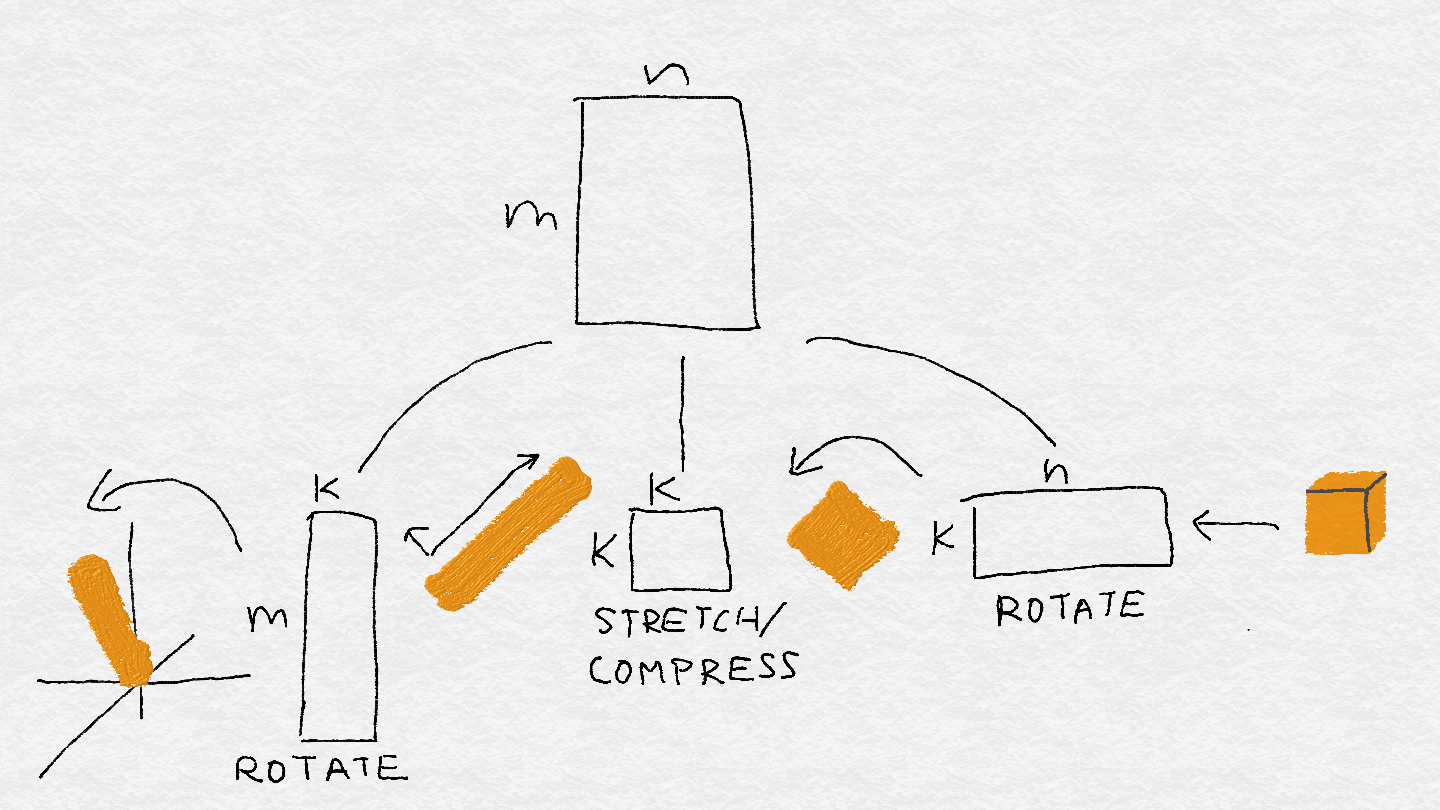
A singular value can be positive, negative, or zero. The ordered set of singular values of a matrix is called its spectrum, and it reveals a lot about the matrix. The gap between the singular values affects how stable the solutions are, and the ratio between the maximum and minimum absolute singular values (the condition number) affects how quickly an iterative solver can find the solution. 奇异值可正、负、零。矩阵的奇异值的有序集合称为它的谱,它揭示了很多关于矩阵的信息。奇异值之间的差距影响解的稳定性,且最大值与最小值的绝对奇异值之比(即条件数)影响迭代找到解的速度。
A.2.1 The Four Fundamental Subspaces of the Data Matrix数据矩阵的四个基本子空间
Another useful way to dissect a matrix is via the four fundamental subspaces: column space, row space, null space, and left null space.
| Mathematical definition: 数学定义: |
Mathematical interpretation: 数学解释: |
Data interpretation: 数据解释: |
Basis: 基: |
|
|---|---|---|---|---|
| Column space 列空间 |
The set of output vectors s where $s = A w$ as we vary the weight vector w. 输出向量集s,对所有权重向量w有$s = A w$。 |
All possible linear combinations of columns. 列的所有线性组合。 |
All outcomes that are linearly predictable based on observed features. The vector w contains the weight of each feature. 根据观察到的特征,所有结果都是线性可预测的。向量w包含每个特征的权重。 |
The left singular vectors corresponding to nonzero singular values (a subset of the columns of U). 对应于非零奇异值的左奇异向量(U列的子集)。 |
| Row space 行空间 |
The set of output vectors r where $r = u^T A$ as we vary the weight vector u. 输出向量集r,对所有权重向量u有$r = u^T A$。 |
All possible linear combinations of rows. 行的所有线性组合。 |
A vector in the row space is something that can be represented as a linear combination of existing data points. Hence, this can be interpreted as the space of “non-novel” data. The vector u contains the weight of each data point in the linear combination. 行空间中的向量可以表示为现有数据点的线性组合。因此,这可以解释为非新奇数据的空间。向量u包含线性组合中每个数据点的权重。 |
The right singular vectors corresponding to nonzero singular values (a subset of the columns of V). 对应于非零奇异值的右奇异向量(V列的子集)。 |
| Null space 零空间 |
The set of input vectors w where $A w = 0$. 输入向量w,满足$A w = 0$。 |
Vectors that are orthogonal to all rows of A. The null space gets squashed to zero by the matrix. This is the “fluff” that adds volume to the solution space of $A w = y$. 与A的所有行正交的向量。零空间被矩阵压到零。这是使$A w = y$的解空间增加体积的绒毛。 |
“Novel” data points that cannot be represented as any linear combination of existing data points. 不能表示为现有数据点的任何线性组合的新数据点。 |
The right singular vectors corresponding to the zero singular values (the rest of the columns of V). 对应于零奇异值的右奇异向量(V的其余列)。 |
| Left null space 左零 空间 |
The set of input vectors u where $u^T A = 0$. 输入向量u 满足$u^T A = 0$ |
Vectors that are orthogonal to all columns of A. The left null space is orthogonal to the column space. 与A的所有列正交的向量。左零空间与列空间正交。 |
“Novel feature vectors" that are not representable by linear combinations of existing features. 不能用现有特征的线性组合表示的新特征向量。 |
The left singular vectors corresponding to the zero singular values (the rest of the columns of U). 对应于零奇异值的左奇异向量(U的其余列)。 |
Column space and row space contain what is already representable based on observed data and features. Those vectors that lie in the column space are non-novel features. Those vectors that lie in the row space are non-novel data points.
For the purposes of modeling and prediction, non-novelty is good. A full column space means that the feature set contains enough information to model any target vector we wish. A full row space means that the different data points contain enough variation to cover all possible corners of the feature space. It’s the novel data points and features—respectively contained in the null space and the left null space—that we have to worry about.
In the application of building linear models of data, the null space can also be viewed as the subspace of “novel” data points. Novelty is not a good thing in this context.
The null space is orthogonal to the row space. It’s easy to see why. The definition of null space states that w has an inner product of 0 with every row vector in A. Therefore, w is orthogonal to the space spanned by these row vectors, i.e., the row space. Similarly, the left null space is orthogonal to the column space.
A.3 Solving a Linear System解线性系统
Let’s tie all this math back to the problem at hand: training a linear classifier, which is intimately connected to the task of solving a linear system. We look closely at how a matrix operates because we have to reverse engineer it. In order to train a linear model, we have to find the input weight vector w that maps to the observed output targets y in the system $A w = y$, where A is the data matrix.让我们把这些数学问题与手头的问题联系起来:训练一个线性分类器,它与求解一个线性系统的任务密切相关。我们仔细观察矩阵是如何运作的,因为我们必须逆向工程它。为了训练一个线性模型,我们需要在系统$A w = y$中找到映射到观测输出目标y的输入权重向量w,其中A是数据矩阵。
Let’s try to crank the machine of the linear operator in reverse. If we had the SVD decomposition of A, then we could map y onto the left singular vectors (columns of U), reverse the scaling factors (multiply by the inverse of the nonzero singular values), and finally map them back to the right singular vectors (columns of V). Ta-da! Simple, right?让我们试着把线性算子的机器反向转动。如果我们有A的SVD分解,那么我们可以将y映射到左边的奇异向量(U的列),反转缩放因子(乘以非零奇异值的倒数),最后将它们映射回右边的奇异向量(V的列)。
This is in fact the process of computing the pseudo-inverse of A. It makes use of a key property of an orthonormal basis: the transpose is the inverse. This is why SVD is so powerful. (In practice, real linear system solvers do not use the SVD, because it’s rather expensive to compute. There are other, much cheaper ways to decompose a matrix, such as QR or LU or Cholesky decompositions.)这实际上是计算A的伪逆矩阵的过程。它利用了标准正交基的一个关键性质:转置是逆。这就是SVD如此强大的原因(实际上,真正的线性系统求解器不使用SVD,因为它的计算成本相当高。还有其他更便宜的方法来分解矩阵,比如QR分解、LU分解或Cholesky分解。)。
However, we skipped one tiny little detail in our haste. What happens if the singular value is zero? We can’t take the inverse of 0 because 1/0 = ∞. This is why it’s called the pseudo-inverse. (The real inverse isn’t even defined for rectangular matrices. Only square matrices have them, as long as all of the eigenvalues are nonzero.) A singular value of zero squashes whatever input was given; there’s no way to retrace its steps and come up with the original input.然而,我们在匆忙中忽略了一个小细节。如果奇异值为0会发生什么?不能求0的倒数因为1/0 = ∞。这就是叫伪逆矩阵的原因(实逆对于矩形矩阵甚至没有定义。只有方阵有它们,只要所有特征值不为零。)。一个为零的奇异值,不管输入是什么;没有办法重新跟踪它的步骤并得到原始输入。
Okay, going backward we get stuck on this one little detail. Let’s take what we’ve got and go forward again to see if we can unjam the machine. Suppose we came up with an answer to $A w = y$. Let’s call it $w_particular$, because it’s particularly suited for y. Suppose that there are also a bunch of input vectors that A squashes to zero. Let’s take one of them and call it $w_sad-trumpet$, because wah wah. Then, what do you think happens when we add $w_particular$ to $w_sad-trumpet$?好了,我们回到这个小细节上。让我们把已有的东西拿出来,再往前走,看看能不能把机器拆开。假设我们得到了$A w = y$的一个答案。叫它$w_particular$,因为是适合y的一个特定解。假设还有一些输入向量A将它们压缩为零。叫它$w_sad-trumpet$。将$w_particular$和$w_sad-trumpet$相加会发生什么? $$A (w_particular + w_sad-trumpet) = y$$ Amazing! So this is a solution too. In fact, any input that gets squashed to zero could be added to a particular solution and give us another solution. The general solution looks like this:神奇!所以这也是一个解。事实上,任何压缩为零的输入都可以加到一个特解中并给出另一个解。通解是这样的: $$w_general = w_particular + w_homogeneous$$ $w_particular$ is an exact solution to the equation $A w = y$. There may or may not be such a solution. If there isn’t, then the system can only be approximately solved. If there is, then y belongs to what’s known as the column space of A. The column space is the set of vectors that A can map to, by taking linear combinations of its columns.$w_particular$是$A w = y$的特解。可能有也可能没有这样的解决方案。若没有特解,系统只有近似解。若有特解,那y属于A的列空间。列空间是A可以通过它的列的线性组合,映射到的向量的集合。 $w_homogeneous$ is a solution to the equation $A w = 0$. (The grown-up name for $w_sad-trumpet$ is $w_homogeneous$.) This should now look familiar. The set of all $w_homogeneous$ vectors forms the null space of A. This is the span of the right singular vectors with singular value 0.$w_homogeneous$是$A w = 0$的解($w_sad-trumpet$更合适的名字是$w_homogeneous$.)。应该对这很熟悉了。所有$w_homogeneous$向量的集合组成A的零空间。这是右奇异向量跨越的空间,其奇异值为0。
The name “null space” sounds like the destination of woe for an existential crisis. If the null space contains any vectors other than the all-zero vector, then there are infinitely many solutions to the equation $A w = y$. Having too many solutions to choose from is not in itself a bad thing. Sometimes any solution will do. But if there are many possible answers, then there are many sets of features that are useful for the classification task. It becomes difficult to understand which ones are truly important.零空间这个名字听起来像是存在危机的目的地。如果零空间包含除全零向量以外的任何向量,那么对于方程$A w = y$有无穷多个解。有太多的解决方案可供选择本身并不是一件坏事。有时候任何解决方案都可以。但是,如果有许多可能的答案,那么对于分类任务来说就有许多有用的特征集。很难理解哪些是真正重要的。
One way to fix the problem of a large null space is to regulate the model by adding additional constraints:解决大零空间问题的一种方法是通过添加额外的约束来规范模型: $A w = y$, where w is such that $w^T w = c$.这里w满足$w^T w = c$。
This form of regularization constrains the weight vector to have a certain norm, c. The strength of this regularization is controlled by a regularization parameter, which must be tuned, as is done in our experiments.这种形式的正则化约束使权重向量具有一定的范数c。这种正则化的强度是由一个正则化参数控制的,这个参数必须进行调整,正如我们在实验中所做的那样。
In general, feature selection methods deal with selecting the most useful features to reduce computation burden, decrease the amount of confusion for the model, and make the learned model more unique. This is the focus of “Feature Selection”.一般来说,特征选择方法是选择最有用的特征,以减少计算量,减少模型的混乱量,使学习的模型更加独特。这是“特征选择”的关注点。
Another problem is the “unevenness” of the spectrum of the data matrix. When we train a linear classifier, we care not only that there is a general solution to the linear system, but also that we can find it easily. Typically, the training process employs a solver that works by calculating a gradient of the loss function and walking downhill in small steps. When some singular values are very large and others very close to zero, the solver needs to carefully step around the longer singular vectors (those that correspond to large singular values) and spend a lot of time digging around in the shorter singular vectors to find the true answer. This “unevenness” in the spectrum is measured by the condition number of the matrix, which is basically the ratio between the largest and the smallest absolute value of the singular values.另一个问题是数据矩阵谱的不均匀性。当我们训练一个线性分类器时,我们不仅关心线性系统是否有通解,还关心是否很容易找到它。通常情况下,训练过程使用一个求解器,它通过计算损失函数的梯度和以小的步骤顺着损失函数走下坡来工作。当某些奇异值非常大而另一些非常接近于0时,解方程需要仔细地遍历较长的奇异向量(那些与较大的奇异值对应的向量),并花费大量时间在较短的奇异向量中寻找真正的答案。这种谱上的不均匀性是由矩阵的条件数来测量的,矩阵的条件数基本上就是奇异值的最大值和最小值的绝对值之比。
To summarize, in order for there to be a good linear model that is relatively unique, and in order for it to be easy to find, we wish for the following: The label vector can be well approximated by a linear combination of a subset of features (column vectors). Better yet, the set of features should be linearly independent.总之,为了有一个相对唯一的好的线性模型,为了它容易找到,我们希望有以下几点:标签向量可以通过特征子集(列向量)的线性组合很好地近似表示。更好的是,特征集应该是线性无关的。
In order for the null space to be small, the row space must be large. (This is due to the fact that the two subspaces are orthogonal.) The more linearly independent the set of data points (row vectors), the smaller the null space.为了使零空间小,行空间必须大(这是由于这两子空间正交)。数据点集(行向量)的线性独立性越强,零空间越小。
In order for the solution to be easy to find, the condition number of the data matrix—the ratio between the maximum and minimum singular values—should be small.为了便于求解,数据矩阵的条件数即最大值与最小奇异值之比应小。